Closed-Form Estimations of the Bistable Region in Metal Cutting via the Method of Averaging

(1)

Closed-Form Estimations of the Bistable Region in Metal Cutting via the Method of Averaging

Tamas G. Molnar^a,∗, Tamas Insperger^b, Gabor Stepan^a

aDepartment of Applied Mechanics, Budapest University of Technology and Economics, H-1111 Budapest, Hungary

bDepartment of Applied Mechanics, Budapest University of Technology and Economics and MTA-BME Lend¨ulet Human Balancing Research Group, H-1111 Budapest, Hungary

Abstract

Machine tool vibrations in turning processes are analyzed by taking into account the nonlinearity of the cutting force characteristics. Unstable limit cycles are computed for the governing nonlinear delay-differential equation in order to determine the bistable technological parameter region where stable stationary cutting and large-amplitude machine tool vibrations coexist. Simple closed- form formulas are derived for the amplitude of limit cycles and for the size of the bistable region considering a general cutting force characteristics. The analytical results are determined by the method of averaging, which can be used to treat the nonlinearities without their third-order approximation. The results are confirmed by numerical continuation and using Melnikov’s integral.

Keywords: machine tool chatter, nonlinear dynamics, bistability, averaging

1. Introduction

Understanding the dynamics of harmful machine tool vibrations (chatter) during metal cutting has been of interest since the 1950’s. Chatter produces noise, reduces the quality of the machined surface, increases tool wear, and may even dam- age the machine tool and/or the workpiece, hence it must be avoided or suppressed. According to the works of Tobias [1]

and Tlusty [2], one main source of machine tool vibrations is the so-called surface regeneration effect: the vibrations of the tool are copied onto the machined surface during metal cutting, which then excite the vibrations in the subsequent cut. This leads to the regeneration of the waviness of the machined surface during the consecutive cuts.

Since the actual vibrations depend on the vibrations recorded on the surface at the previous cut, the dynamics of machine tool chatter is described by delay-differential equations (DDEs).

Turning or drilling processes are typically described by autonomous DDEs, while milling can be modeled by time- periodic DDEs [3, 4, 5, 6, 7, 8, 9, 10]. In what follows, we restrict ourselves to autonomous equations. The DDEs governing machine tool chatter are typically nonlinear, since the cutting force is a nonlinear function of the chip thickness [7].

Machine tool vibrations can be explained by the instability of the stationary solution (equilibrium) of the nonlinear (autonomous) DDE. The (in)stability is conventionally illustrated in stability lobe diagrams. These are depicted in the plane of the most important technological parameters – the spindle speed

∗Corresponding author

Email addresses:molnar@mm.bme.hu(Tamas G. Molnar ), insperger@mm.bme.hu(Tamas Insperger),stepan@mm.bme.hu(Gabor Stepan)

and the depth or the width of cut – and distinguish the regions associated with stable machining from those of machine tool chatter. When chatter occurs, the stability of stationary cutting (the equilibrium) is lost via Hopf bifurcation. According to [11, 12, 13, 14], the Hopf bifurcation is typically subcritical and gives rise to an unstable periodic orbit (limit cycle) in the vicinity of the linearly stable equilibrium. Therefore, there exists a region of bistability [15, 14, 16, 17, 18, 19] where the basin of attraction of the linearly stable equilibrium does not cover the whole phase space and chatter occurs to large enough perturbations. Here, stable stationary cutting coexists with large-amplitude chatter, hence this region is unsafe and preferably must be avoided.

In this paper, we focus on computing the limit cycle and the bistable technological parameter region for turning processes.

Since the phase space of DDEs is infinite dimensional [20], such analysis is nontrivial, although there exist several analytical approaches to compute limit cycles for nonlinear DDEs.

The two most popular methods are center manifold reduction [21, 22, 23, 24, 25] and the method of multiple scales [26], but there exist several other approaches such as the method of small parameters [26, 27], harmonic balance [16, 28], or Mel- nikov’s integral [29]. For orthogonal cutting models, center manifold reduction is discussed in [11, 12, 13, 14], while the method of multiple scales is presented in [30, 31, 32]. These analyses are typically restricted to a cubic approximation of the nonlinearity, since higher-order terms lead to extremely long and difficult expressions.

In this paper, we use the method of averaging [33, 34, 35, 36, 37, 38, 39, 40, 41] to compute the periodic orbit. This method can easily be employed for higher-order nonlinearities, however, the analysis involves less rigorous derivations than the center manifold reduction or the method of multiple scales. The

(2)

m

c k

feed

q(t) h(t) q q(t−t)

h₀ x

0 q

tool

workpiece

F

0

a W

q q

q

Figure 1: Single-degree-of-freedom mechanical model of turning.

results obtained below are valid only if the periodic solution of the nonlinear DDE is close to harmonic. We show that this condition is satisfied for the most typical cutting force expressions.

Note that extensions of the averaging method to use explicitly given non-harmonic periodic expressions also exist, see for example [29, 42]. We also demonstrate that the same analysis could be conducted alternatively by Melnikov’s integral, and we verify the analytical results by numerical continuation.

The rest of the paper is organized as follows. The mechanical model of turning processes with the governing DDE is presented in Sec. 2. Linear stability analysis and the phenomenon of bistability are reviewed in Sec. 3 based on the existing literature. The method of averaging is used in Sec. 4 to derive simple approximate analytical formulas for the amplitude of periodic solutions in Sec. 5 and for the size of the bistable region in Sec. 6. Discussion and comparison to other approaches are presented in Sec. 7.

2. Mechanical Model

Consider the mechanical model of turning processes shown in Fig. 1. We assume that the workpiece is rigid, the tool is compliant and its vibrations can be described by a single dominant vibration mode that takes place along the feed direction.

The equation governing the tool’s motion is

¨

q(t)+2ζωnq(t)˙ +ω²_nq(t)= 1 mq

Fq(h(t),a), (1) wherem_qis the modal mass,ωnis the undamped natural angular frequency andζis the damping ratio of the dominant vibration mode described by the generalized coordinateq.

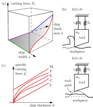
Fq denotes the generalized force that is the q-directional component of the cutting force acting on the tool. It is typically proportional to the chip widthaand depends on the uncut chip thicknessh[7], see Fig. 2(a). This is expressed by

Fq(h,a)=











a f_q(h) ifh>0,

0 ifh≤0, (2)

cutting force Fq

chip width a

chip thickness h speciﬁc

cutting force fq

L C E P SL (a)

(c)

chip thick-

ness h m

c k

tool

q q

q

m

c k

tool

q q

q

h(t)>0

h(t)<0 (b)

workpiece

workpiece tool-

path

Figure 2: (a) Characteristics (2) of the cutting force; (b) illustration of the flyover effect; (c) models (3)-(7) of the specific cutting force [43].

where the specific cutting force f_q(h) is a function of the uncut chip thicknessh. The caseh≤0 occurs if the tool jumps out of the workpiece and loses contact with the material due to large- amplitude vibrations. In such cases, the cutting force becomes zero. This phenomenon is called flyover and is illustrated in Fig. 2(b). In what follows, we restrict ourselves to cases where the tool remains in contact with the workpiece during machining.

The relationship between the specific cutting force fq and the uncut chip thicknessh can be described by various models, see [43] and the references therein. The most widely ac- cepted expressions are the linear (L) and shifted linear (SL) functions [7], the power law (P) [44, 7], the cubic polynomial (C) [15] and the exponential (E) cutting force characteristics [45] that are given by

f_q^L(h)=Kch, (3)

f_q^SL(h)=Ke+Kch, (4)

f_q^P(h)=Kνh^ν, (5)

f_q^C(h)=ρ1h+ρ2h²+ρ3h³, (6) f_q^E(h)=b1h+b2

b3

e^b³^h+b4, (7) respectively. Here, K_e,c, K_ν, ν, ρ_1,2,3, b_1,2,3,4 are parameters that can be obtained from experimental cutting force measure- ments. The specific cutting force models (3)-(7) are illustrated in Fig. 2(c). Now, we focus on the nonlinear expressions: we analyze the power law (5), the cubic polynomial (6) and the exponential function (7) in detail.

According to the theory of regenerative machine tool chatter [1, 2], the instantaneous uncut chip thicknessh(t) is deter-

(3)

mined by the actual tool positionq(t) and the positionq(t−τ) of the previous cut taking place one workpiece revolution before.

Therefore,

h(t)=h0+q(t−τ)−q(t), (8) whereh0is the prescribed chip thickness (feed per revolution).

Parameter τis called the regenerative delay. It is equal to the rotational period and is related to the angular velocityΩof the workpiece byτ=2π/Ω.

Equations (1), (2) and (8) form a nonlinear delay-differential equation. This equation has a unique equilibriumq(t)≡q₀that can be given in the form

q0= a fq(h0)

mqω²_n . (9)

The equilibrium describes the ideal (chatter-free) machining: stationary cutting with constant prescribed chip thickness h(t)≡h0. The onset of machine tool chatter is associated with the instability of the equilibrium. In order to analyze stability, we introduce the dimensionless coordinate

x(t)= q(t)−q0

h₀ . (10)

We also use the dimensionless time ˜t=ωntand the dimensionless delay ˜τ=ωnτ. The derivative with respect to ˜tis indicated by prime and satisfies ˙x(t)=ωnx⁰(˜t). After dropping the tildes, we obtain

x⁰⁰(t)+2ζx⁰(t)+x(t)= a mqω²_n

fq(h(t))−fq(h₀) h0

, (11) whereh(t) is given by Eq. (8) and can be expressed using coor- dinatexvia Eq. (10).

Now, we expand f_q(h(t)) into Taylor series aroundh₀: fq(h(t))=

∞

X

m=0

1

m!f_q^(m)(h0)h^m₀(x(t−τ)−x(t))^m. (12) Substitution of Eq. (12) into Eq. (11) yields the dimensionless equation of motion in the form

x⁰⁰(t)+2ζx⁰(t)+x(t)=w

∞

X

m=1

ηm(x(t−τ)−x(t))^m, (13)

where the expressions of the dimensionless chip widthw(that is proportional to the actual chip widtha) and the dimensionless cutting force coefficientsηmread

w=a f_q⁰(h0)

mqω²_n , (14)

η_m= 1 m!

fq^(m)(h0)

f_q⁰(h₀) h^m−1₀ , m∈Z⁺. (15) Note thatη1=1.

3. Linear Stability and Bistability

Via linear stability analysis [46], it can be shown that the machining is stable for chip widths 0 < w < wH. The linear stability boundaries can be obtained via D-subdivision [46] by substituting the trial solution x(t)= Xe^iωt,X ∈ C\{0}into the linear part of Eq. (13), separating real and imaginary parts, and solving

−ω²+1+w(1−cos(ωτ))=0,

2ζω+wsin(ωτ)=0, (16) which leads to [46]

wH(ω)=

ω²−12

+4ζ²ω² 2 ω²−1 , τH(ω,j)= 2

ω jπ−arctan ω²−1 2ζω

!!

, ΩH(ω,j)= 2π

τH(ω,j).

(17)

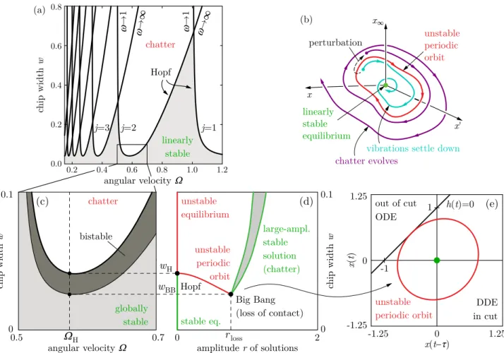
Equation (17) defines a family of curves called stability lobes with lobe number j∈N. The curves are parameterized by ω ∈ (0,∞). The stability lobes are conventionally depicted in the plane of the technological parameters such as the (dimensionless) angular velocityΩand the (dimensionless) chip width w, which results in so-called stability lobe diagrams (or stability charts) as shown in Fig. 3(a) forζ = 0.02. Gray shading indicates the linearly stable region 0<w <w_Hthat is associated with chatter-free cutting process. The stability charts help manufacturing engineers in the selection of optimal technological parameters where machine tool chatter is avoided and the material removal rate (proportional toΩw) is high.

Along the linear stability boundaries (17), Hopf bifurcation occurs (as indicated by subscript H). The theory of Hopf bifurcation in delay-differential equations is covered by [21, 22, 23, 20, 24], while its analysis for turning processes can be found in [11, 12, 13, 14]. According to [14], the Hopf bifurcation is subcritical for the power law (5) and for the cubic cutting force characteristics (6) with realistic parameters. The subcriticality implies that the Hopf bifurcation gives rise to an unstable periodic orbit (unstable limit cycle) in the vicinity of the linearly stable equilibrium. The approximate dimensionless angular frequency of the limit cycle isω∈(0,∞).

This phenomenon is illustrated qualitatively in Fig. 3(b) where the phase portrait of Eq. (13) is depicted. Although the phase space of Eq. (13) is infinite-dimensional, the trajectories can still be illustrated using three coordinates: x, x⁰ andx∞, wherex_∞refers to the remaining infinite dimensions. Accord- ing to Fig. 3(b), the basin of attraction of the linearly stable equilibrium does not cover the whole phase space when the unstable limit cycle exists, thus the equilibrium is not stable in the global sense. Depending on initial conditions and perturbations (such as material inhomogeneity or external excitation), the system may leave the basin of attraction and converge to another stable solution. This solution is large-amplitude chatter

(4)

angular velocity W

chip width w

amplitude r of solutions 0.1

00.5

0.7 chatter

globally stable

chip width w

0.1

stable eq. 0 unstable equilibrium

unstable periodic orbit

large-ampl.

stable solution (chatter)

Big Bang (loss of contact)

0 2

Hopf w_H w_BB

r_loss bistable

(d) (c)

WH

1.25

-1.25

-1.25 1.25

x(t t)

x(t)

DDE in cut out of cut

ODE

h(t)=0 (e)

0 0 -1

1 (b)

perturbation unstable

periodic orbit

linearly stable equilibrium

vibrations settle down chatter evolves

x

x'

∞

(a)

w→∞

w→∞ w→1

w→1

j=2 Hopf

j=1 j=3

chatter

linearly stable

chip width w

0.0 0.2 0.4 0.6 0.8

1.2 1.0

0.2 0.4 0.8

angular velocity W 0.6

Figure 3: (a) Stability lobe diagram of turning; (b) illustration of the trajectories near the unstable periodic orbit arising from Hopf bifurcation; (c) illustration of the bistable region; (d) the corresponding bifurcation scenario; (e) the periodic orbit at loss of contact.

– an intermittent motion where the tool leaves and gets back into the workpiece repeatedly [11, 12, 13, 47, 14, 48].

The parameter domain where stable stationary cutting and large-amplitude chatter coexist due to the existence of an unstable periodic orbit is referred to as region of bistability (or unsafe zone). It is important to emphasize that the phenomenon of bistability is caused by the nonlinearity in the system. If a linear cutting force characteristics (i.e. η_m=0 form≥2) was considered in Eq. (13), then the bistable region would disap- pear. However, the existence of the bistable region was verified experimentally in [12, 49, 16, 43], while its numerical analysis for milling was published in [19]. From practical point of view, bistability should be avoided, since chatter may occur de- spite linear stability if the cutting process is perturbed as illustrated in Fig. 3(b). The bistable region is shown qualitatively in Fig. 3(c) with dark grey shading. Light grey shading indicates the globally stable region, where the cutting process is safe and no machine tool vibrations evolve.

The corresponding bifurcation scenario is discussed in [48]

in detail and is illustrated in Fig. 3(d). The bifurcation parameter is chosen to be the dimensionless chip widthw, while the dimensionless angular velocityΩ = ΩHis fixed (see the dashed line in Fig. 3(c)). As shown by Fig. 3(d), the amplituder of the unstable limit cycle born from Hopf bifurcation increases

with decreasing bifurcation parameter. At the critical ampli- tuderloss, the (unstable) oscillations get so large that the tool loses contact with the workpiece as illustrated in Fig. 1(b). In such cases, the chip thickness drops to zero and to negative val- ues (h(t)≤0) that is associated with nonsmoothness in the cutting force characteristics (2) and with nonsmooth dynamics: the governing equation switches from a delay-differential equation to an ordinary differential equation. The unstable periodic orbit corresponding torlossis illustrated in Fig. 3(e).

According to [48], the unstable periodic orbit undergoes a special nonsmooth fold bifurcation (called Big Bang bifurcation) atrloss. The nonsmooth fold gives rise to a large-amplitude stable solution that corresponds to machine tool chatter, which may be a periodic or chaotic motion that is stable in the dynamical sense [48]. Thus, the linearly stable equilibrium coexists with the large-amplitude stable solution between the Hopf bifurcation pointw = wHand the Big Bang bifurcation point w=wBB, see Fig. 3(d). The bistable region iswH<w<wBB, and its boundaryw=wBBcan be obtained by locating the point where the unstable periodic solution first satisfies the condition h(t)=0 associated with loss of contact, cf. Fig. 3(e).

The rest of the paper deals with the computation of the unstable limit cycle and the bistable region. In [11, 12, 13, 14], approximate analytical formulas were given for the bistable re-

(5)

gion. These analyses used a cubic (expansion of the) cutting force characteristics and were valid in the vicinity of Hopf bifurcation only. Thus, the formulas for the bistable region are inaccurate in some cases (for large bistable regions or in the presence of higher-order nonlinearities). The rest of the paper is devoted to extending these results by the derivation of more accurate analytical formulas for the bistable region while considering higher-order nonlinearities. A similar effort can be found in [16] for the power law (5) – now we consider a general cutting force characteristics.

4. Method of Averaging

In order to compute the bistable region, the amplitude of the unstable limit cycle must be determined. In what follows, we use the Krylov-Bogoliubov-Mitropolsky method of averaging [33] to find the amplitude. The key point of the analysis is the approximation of the limit cycle by its first harmonic. At Hopf bifurcation (w = wH), the linear part of Eq. (13) indeed has harmonic solution. The linear part reads

x⁰⁰(t)+2ζx⁰(t)+x(t)=wH(x(t−τ)−x(t)), (18) whereas its solution can be given in the form

x(t)=rcos(ωt+ϕ),

x⁰(t)=−rωsin(ωt+ϕ), (19) where the amplituderand the phaseϕdepend on initial conditions. The solution of the nonlinear system (13) is sought for in the same form as in Eq. (19), but with time-dependent amplitude ˆr(t) and phase ˆϕ(t):

x(t)=ˆr(t) cos(ωt+ϕ(t))ˆ ,

x⁰(t)=−ˆr(t)ωsin(ωt+ϕ(t))ˆ . (20) The constant approximation of ˆr(t) and ˆϕ(t) implies the harmonic approximation of the limit cycle. Thus first, we trans- form Eq. (13) and express it in terms of ˆr(t) and ˆϕ(t). Then, we search for constant (approximate) solutions.

By multiplying the left-hand side of the expressions in Eq. (20) by cos(ωt+ϕ(t)) andˆ −sin(ωt+ϕ(t))/ω, respectively,ˆ and by adding them, we get the amplitude as

ˆ

r(t)=x(t) cos(ωt+ϕ(t))ˆ −x⁰(t)1

ωsin(ωt+ϕ(t))ˆ , (21) while the following identity can also be obtained in a similar manner:

0≡x(t) sin(ωt+ϕ(t))ˆ +x⁰(t)1

ωcos(ωt+ϕ(t))ˆ . (22) Differentiation of Eq. (21) with respect to time and using Eqs. (13) and (22) yields the Lie derivative of the amplitude ˆ

r(t) in the form rˆ⁰(t)=−1

ω

ω²x(t)−2ζx⁰(t)−x(t) +w

∞

X

m=1

η_m(x(t−τ)−x(t))^m

sin(ωt+ϕ(t))ˆ . (23)

Similarly, the Lie derivative of the phase ˆϕ(t) can be expressed via differentiation of Eq. (22) and using Eqs. (13) and (21), which gives

ϕˆ⁰(t)= 1 ωˆr(t)

ω²x(t)−2ζx⁰(t)−x(t) +w

∞

X

m=1

ηm(x(t−τ)−x(t))^m

cos(ωt+ϕ(t))ˆ . (24)

From this point on, Eq. (23) is considered only to calculate the bistable region from the amplitude of the limit cycle.

Now, we make the main assumption of the subsequent analysis. We suppose that the amplitude ˆr(t) and the phase ˆϕ(t) vary slowly in time (which is reasonable as we seek for their constant approximation). Note that this can also be considered as a multiple scales assumption. The slow variation implies ˆ

r(t−τ)≈r(t) and ˆˆ ϕ(t−τ) ≈ ϕ(t). Then, the chip thicknessˆ variationx(t−τ)−x(t) in Eq. (23) can be approximated using Eq. (20) as

x(t−τ)−x(t)≈r(t)ˆ r

4 sin² ωτ

2

cos(ωt+ϕ(t)ˆ +ψ), (25)

whereψis a phase shift satisfying sinψ=− sin(ωτ)

r 4 sin²

ωτ 2

. (26)

Substituting Eqs. (20) and (25) into Eq. (23) leads to the differential equation for ˆr(t) in the form

ˆ

r⁰(t)=−2ζr(t) sinˆ ²(ωt+ϕ(t))ˆ + 1

ω −ω

!

r(t) cos(ωtˆ +ϕ(t)) sin(ωtˆ +ϕ(t))ˆ

− 1 ωw

∞

X

m=1

η_mr^m(t)

4 sin² ωτ

2 m/2

×cos^m(ωt+ϕ(t)ˆ +ψ) sin(ωt+ϕ(t))ˆ . (27) Notice that Eq. (27) is a nonautonomous ordinary differential equation that does not involve time delay anymore.

Now, the method of averaging is applied to Eq. (27). The the- oretical background and examples for this method can be found in [33, 34, 35, 36, 37, 38, 39, 40, 41]. Equation (27) is averaged by integrating both sides from 0 to 2π/ωwith respect totwhile considering ˆrand ˆϕtime-independent. Multiplying the resulting equation byω/(2π), the averaged system is obtained in the form

r⁰(t)=−ζr(t)− w 2πω

∞

X

m=1

η_mr^m(t)

4 sin² ωτ

2 m/2

β_m, (28)

whereris the averaged amplitude andβ_mis defined by βm=Z 2π/ω

0

cos^m(ωt+ψ) sin(ωt)ωdt, m∈Z⁺. (29)

(6)

Note that the phase ˆϕis omitted inβm, since a phase shift does not modify the integral of a periodic function over its time period. The expression ofβ_mcan be simplified to

β2k−1=−πsinψ 4^k−1

2k−1 k

!

, β2k=0, k∈Z⁺. (30)

5. Amplitude of the Limit Cycle

Consider the constant approximation ˆr(t) ≈ r(t) ≈ rof the amplitude that corresponds to the harmonic approximation of the limit cycle. Substitution of r(t) ≡ r and Eq. (30) into Eq. (28) gives

−ζr+ w 2πω

∞

X

k=1

η_2k−1r^2k−1

×

4 sin² ωτ

2

(2k−1)/2πsinψ 4^k−1

2k−1 k

!

=0. (31) Now, we substituteζfrom Eq. (16), we use Eq. (26) and divide byrsin(ωτ)/(2ω),0. These yield

wH−w

∞

X

k=1

2k−1 k

! η2k−1

r²sin²

ωτ 2

k−1

=0. (32) The calculation of the approximate amplituderof the periodic orbit is reduced to finding a positive real root of the polynomial in Eq. (32). If the nonlinearity in Eq. (13) is a polynomial of low order, then Eq. (32) can be solved analytically for r²sin²(ωτ/2) to obtainr. The cubic cutting force characteristics (6), that is,ηm=0 form≥4 leads to

r3rd(w)= vu

t− w−wH

3η3sin² ωτ

2

w

. (33)

For quintic nonlinearity (ηm=0 form≥6), Eq. (32) gives

r5th(w)= vu uu uu

ut−3η3w+ q

9η²₃w²−40η5w(w−wH) 20η5sin²

ωτ 2

w

. (34)

In a similar manner, Eq. (32) can be solved analytically by computer algebra for 7th, 9th and 11th-order nonlinearities as well, but the resulting formulas are too long to be listed here.

Above 11th order and for complete Taylor series, Eq. (32) can be solved numerically for the amplitude.

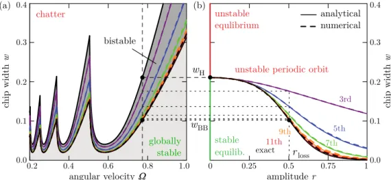
The amplituderof the limit cycle as a function of the dimensionless chip widthwis shown in Fig. 4(b). Here, the damping ratio is ζ = 0.02 and the bifurcation diagrams are computed forΩ = 0.77486 (i.e., j =2,ω= 1.1903) as indicated by the dashed line in the corresponding stability chart in Fig. 4(a). The exponential cutting force characteristics (5) is considered with feed per revolution h0 = 0.05 mm. The cutting coefficients areb1 =176 N/mm²,b2 =4386 N/mm³,b3 =−129 1/mm, b4=0, which were identified in [50] for milling aluminum with four cutting teeth. In order to show the effect of higher-order

nonlinear terms, the nonlinearity in Eq. (13) is truncated after the 3rd, 5th, 7th, 9th and 11th-order terms as shown by purple, blue, green, orange and red colors, respectively. The analytical bifurcation diagrams obtained from Eq. (32) are indicated by solid lines. The amplitude corresponding to the full nonlinear term in Eq. (13) is shown by black color. This black curve was obtained by simplifying the sum in Eq. (32) to a closed-form expression via computer algebra and by creating a contour plot based on Eq. (32) afterwards.

The analytical results were verified by numerical continuation using DDE-Biftool[51]. The numerical bifurcation diagrams showing half of the peak-to-peak amplitude of the limit cycle are indicated by dashed lines with the same color scheme as that of their analytical counterparts. The analytical and numerical results agree well, the solid and dashed branches over- lap. This justifies that the periodic solution of Eq. (13) is indeed nearly harmonic.

6. Region of Bistability

Expressions for the amplitude of the limit cycle allow the calculation of the bistable region. Figure 4(b) shows that higher- order nonlinearities have significant effect on the amplitude and hence on the size of the bistable region. Thus, we extend the results of [14] and derive formulas for the size of the bistable region by taking into account the full nonlinear term in Eq. (13).

According to [48], the boundaryw=wBBof the bistable region is located where the amplitude of the unstable periodic oscillations gets so large that the flyover shown in Fig. 1(b) takes place. This happens when the chip thickness drops to zero. The chip thickness h(t) can be expressed using Eqs. (8), (10) and (25). Then, substitution of ˆr(t)≈r and cos(ωt+ϕ(t)ˆ +ψ)=−1 into h(t) = 0 gives the smallest am- plituderlosswhere loss of contact takes place in the form

rloss= 1 r

4 sin² ωτ

2

. (35)

Note that the bifurcation diagrams in Fig. 4(b) are valid for 0≤r≤rlossonly (whererloss=0.503 in this example).

When the chip width is decreased tow = w_BB, the amplitude of the unstable limit cycle becomes rloss. Thus, loss of contact takes place and the boundary of the bistable region is reached. After substitution ofw=wBB,r =rloss and Eq. (35) into Eq. (32), the boundary of the bistable region becomes

wBB=wH







∞

X

k=1

1 4^k−1

2k−1 k

! η_2k−1







−1

. (36)

The size of the bistable region can be compared to the size of the linearly stable region by introducing the ratio

Rbist=wH−wBB

wH

(37)

(7)

(a) chatter

globally stable angular velocity W

chip width w

0.0 0.1 0.2 0.3 0.4

1.0 0.8

0.6 0.4

0.2

(b)

chip width w

0.0 0.1 0.2 0.3 0.4

3rd

11th 7th

5th unstable

equlibrium

stable equilib.

9th

analytical numerical

amplitude r

1 0.75 0.5

0.25 0

exact

wH

wBB

rloss

bistable

Figure 4: (a) Stability chart of the turning model (13); (b) bifurcation diagrams for different orders of nonlinearity. Solid lines indicate analytical results obtained from Eq. (32), dashed lines show the results of numerical continuation by DDE-Biftool.

that can be expressed as Rbist =1−







∞

X

k=1

1 4^k−1

2k−1 k

! η2k−1







−1

=1− 1+3 4η3+10

16η5+35

64η7+126 256η9+. . .

!−1

. (38) Note that the approximate sizeRbistof the bistable region is independent of the location of the Hopf bifurcation point (i.e., independent ofωorΩ). Besides, recall that the bistable region disappears for a linear cutting force characteristics. Accord- ingly, Eq. (38) shows thatRbist=0 ifηm=0 form≥2.

For the power law cutting force characteristics (5), substitution of Eq. (15) into Eq. (38) and simplification give

Rbist=1−

√πΓ(ν+2) 2^ν⁺¹Γ

ν+¹₂, (39) whereΓdenotes the Euler gamma function. For the cubic cutting force characteristics (6), the resulting expression is

Rbist= 3ρ3h²₀

4ρ₁+8ρ₂h₀+15ρ₃h²₀. (40) In the case of the exponential cutting force characteristics (7), the size of the bistable region becomes

Rbist=1− b1h0+b2h0e^b³^h⁰ b₁h₀+2b2

b3

e^b³^h⁰I₁(b₃h₀)

, (41)

whereI₁is the modified Bessel function of the first kind.

Using formulas (38)-(41), the bistable region can be computed analytically as shown by the solid lines in Fig. 4(a). Here, the same color scheme is used as in Fig. 4(b), and the analytical results were again verified by numerical continuation with DDE-Biftool, see the overlapping dashed lines. In what follows, we evaluate formulas (39)-(41) and compare them to existing results in the literature.

7. Results and Discussion

It must be mentioned that formula (39) associated with the power law cutting force characteristics (5) was already derived by Tam´as Kalm´ar-Nagy in [16] and also by Pankaj Wahi according to personal communications [52]. In their works an equivalent approach, the method of harmonic balance was used.

Equation (39) shows that, for the power law, the size of the bistable region depends on the cutting exponentν only. As- sumingν = 3/4 (i.e., the well-known three-quarter rule), the bistable region occupies 6.5% of the linearly stable region. That is, the bistable region is small independently of any technological parameters. For other cutting force characteristics (that were not discussed in [16]), the bistable region is more significant and an accurate closed-form formula for its prediction becomes more relevant. Formula (38) introduced in this paper is valid for any cutting force characteristics.

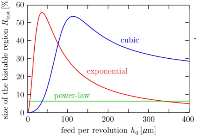
For the cubic polynomial (6) and the exponential cutting force characteristics (7), the bistable region depends on the feed h0 per revolution according to Eqs. (40) and (41). Thus, the bistable region may be significantly larger than 6.5% of the linearly stable region, which was also confirmed by experiments with large feed rates in [43]. The size of the bistable region is plotted against the feed h0 per revolution in Fig. 5 for the power law (green), the cubic polynomial (blue), and the exponential characteristics (red). The cutting force parameters are ν = 3/4 for the power law, ρ1 = 6.1096×10³ N/mm², ρ2 = −5.41416×10⁴ N/mm³, ρ3 = 2.03769×10⁵ N/mm⁴ for the cubic polynomial (that were identified experimentally in [15] for a milling tool of four teeth), andb1 =176 N/mm², b2 = 4386 N/mm³,b3 = −129 1/mm, b4 = 0 for the exponential function (the same as in Fig. 4). For the cubic and the exponential cutting force expressions, the bistable region becomes significant: it occupies about 50% of the linearly stable region at certain critical feed per revolutions.

This justifies the relevance of considering other cutting force characteristics than the power law. To the best knowledge of the

(8)

0 20 30 40 50 60

size of the bistable region R [%]bist

feed per revolution h [mm]₀

400 300

200 100

0 10

exponential cubic

power-law

Figure 5: The size of the bistable region as a function of the feed per revolution for various cutting force characteristics.

authors, the exponential cutting force expression has not been analyzed previously from nonlinear dynamics point of view. On the other hand, the cubic characteristics has been studied exten- sively in the literature. Cubic nonlinearities and bistability in orthogonal cutting were first discussed in [15] via the method of harmonic balance without deriving closed-form formulas for the bistable region. Later, it was analyzed by center manifold reduction in [11, 12, 13, 14] and by the method of multiple scales in [30, 31, 32]. In [14], it was shown that the size of the bistable region occupies approximately 3/4η₃portion of the linearly stable region. These analyses, however, are valid in the vicinity of the Hopf bifurcation only. Farther away, the results become inaccurate and cannot predict the size of a large bistable region accurately (an overestimation by a factor of 2 was reported in [14] at critical feed per revolutions).

In [53], a higher-order estimation for the amplitude of limit cycles was introduced, which is still valid farther from the Hopf bifurcation. This way, the results of [11, 14] could be refined and larger bistable regions could also be predicted accurately.

This method is based on center manifold reduction and uses the property limw→0r = ∞ of the limit cycle (that is also captured by Eqs. (32), (33) and (34)). This approach gives 3/4η3/(1+3/4η3) for the size of the bistable region, which is the same that obtained by averaging, see the truncation of Eq. (38) for cubic nonlinearity.

The method of averaging is not restricted to the cubic approximation of the cutting force characteristics but can be applied to higher-order nonlinearities as well. It should be mentioned, however, that the coefficients of higher-order terms are more uncertain and harder-to-measure from engineering point of view. In the meantime, the experimentally determined size of the bistable zone can be used well for the identification of these higher-order terms by applying the results in an inverse way as shown in [43]. Consideration of higher-order terms is theoretically possible by center manifold reduction and by the method of multiple scales, too, but the calculations become un- manageably complicated.

Note that the approximate solution (20) obtained by the

method of averaging has a certain error and timescale of validity. In order to investigate this error and timescale, let us rewrite Eq. (13) in the form

x⁰⁰(t)+2ζx⁰(t)+x(t)−wH(x(t−τ)−x(t))

=ε





x(t−τ)−x(t)+ w w−wH

∞

X

m=2

η_m(x(t−τ)−x(t))^m





 (42) withε=w−wH. This form satisfies that forε=0 Eq. (42) has the harmonic solution of the form (19). Thus, form (42) reveals that, forε,0, solution (20) has a timescale of validity 1/εand is accurate with errorO(ε) [40]. Here, the timescale of validity is not of importance, because it is associated with the accuracy of the phase ˆϕ(t). Since the amplitude of the unstable limit cycle was required only to obtain the bistable region, the phase was not even determined and its accuracy is irrelevant from practical point of view. As for the amplitude, its error turned out to be practically negligible, see Fig. 4.

Apart from the method of averaging, the amplitude (32) of the limit cycle and the bistable region can also be derived using Melnikov’s integral. This method serves equivalent results to averaging, which is shown in the Appendix for the sake of completeness. The method of averaging and Melnikov’s integral serve rigorous results with the possibility of giving error estimates for the obtained approximate solutions.

In summary, the method of averaging provides simple closed-form formulas for the size of the bistable region in metal cutting even in the presence of higher-order nonlinearities. Nu- merical continuation confirmed the accuracy of the analytical results even at critical feed per revolutions where the bistable region is large. Although the key point of the analysis is the harmonic approximation of the limit cycle, the nonlinearity was expanded into Taylor series as in center manifold reduction.

However, it is not necessary to truncate the series after finitely many terms: it is possible to obtain the size of the bistable region analytically for a complete Taylor series as well, see Eqs. (39) and (41). The amplitude of the limit cycle can be determined analytically for up to 11th-order nonlinearity and numerically for any order using Eq. (32). Whereas the result (38) for the size of the bistable region is analytical for any order of nonlinearity, and this result is relevant from practical point of view.

Acknowledgements

This work has been supported by the ´UNKP-16-3-I. New National Excellence Program of the Ministry of Human Ca- pacities. The research leading to these results has received funding from the European Research Council under the Eu- ropean Union’s Seventh Framework Programme (FP/2007- 2013)/ERC Advanced Grant Agreement n. 340889.

Appendix A. Solution by Melnikov’s Integral

Finally, we show that Eq. (32) for the approximate amplitude of the limit cycle can also be obtained using Melnikov’s integral. This method is discussed in [42] in detail, and its core idea

(9)

is decomposing the dynamical system to a Hamiltonian system and a perturbation. The unperturbed Hamiltonian system is of form

x⁰₁(t)= ∂H

∂x₂(t), x⁰₂(t)=−∂H

∂x₁(t),

(A.1)

where the Hamiltonian H is constant along the trajectories of the system, since its Lie derivative is zero:

H⁰(t)= ^∂H_∂x₁(t)x⁰₁(t)+_∂x^∂H₂(t)x⁰₂(t)≡0. For Eq. (13), the unperturbed Hamiltonian system is given by Eq. (18), thus with x1(t)=x(t) andx2(t)=x⁰(t) the Hamiltonian becomes

H(t)= x²₁(t)ω² 2 +x²₂(t)

2 . (A.2)

The solution of the unperturbed system is given by Eq. (19) and the corresponding trajectories are closed curves in the plane (x1,x2). According to [42], one of these closed trajectories is preserved as a limit cycle in the perturbed nonlinear system, which, in some sense, conserves the property thatHis constant along the closed trajectory.

The perturbed system can be given in the form x⁰₁(t)= ∂H

∂x2

(t)+g₁(t), x⁰₂(t)=−∂H

∂x₁(t)+g₂(t),

(A.3)

where the perturbation is g1(t)=0,

g2(t)=(w−wH)∆x1(t)+w

∞

X

m=2

ηm∆x^m₁(t) (A.4) with ∆x1(t) = x1(t −τ)− x1(t), see Eq. (13). In this perturbed system, the Lie derivative of the associated Hamiltonian isH⁰(t)= ^∂H_∂x₁(t)x⁰₁(t)+^∂H_∂x₂(t)x⁰₂(t)=g2(t)x⁰₁(t)−g1(t)x⁰₂(t). Ac- cording to [42], the condition for a closed trajectory of the unperturbed system (that satisfiesH(t)=const) to be preserved in the perturbed system is given by Melnikov’s integral:

I

L

g2(t)x⁰₁(t)−g1(t)x⁰₂(t)dt=0, (A.5) whereLdenotes the closed trajectory of the perturbed system (i.e., the limit cycle).

Substitution of Eq. (A.4) yields I

L





(w−wH)∆x1(t)+w

∞

X

m=2

ηm∆x^m₁(t)





x⁰₁(t)dt=0. (A.6) Now, we approximate the limit cycle L by the corresponding trajectory of the unperturbed system: we substitute the harmonic solution (19) into Eq. (A.6) and carry out the integration over [0,2π/ω]. We obtain

−(w−w_H)r² r

4 sin² ωτ

2 β₁

−wr

∞

X

m=2

η_mr^m

4 sin² ωτ

2 m/2

β_m=0, (A.7)

whereβmis defined by Eq. (29). Substituting the simplified expression (30) ofβm, Eq. (A.7) becomes equivalent to Eq. (32) obtained by the method of averaging. Consequently, Eq. (32) and all the subsequent equations can alternatively be derived using Melnikov’s integral, while Figs. 4 and 5 can also be obtained by this method.

References

[1] S. A. Tobias, W. Fishwick, Theory of regenerative machine tool chatter, The Engineer (1958) 199–203, 238–239.

[2] J. Tlusty, M. Polacek, The stability of the machine tool against self- excited vibration in machining, in: ASME Production Engineering Re- search Conference, Pittsburgh, PA, USA, 1963, pp. 454–465.

[3] M. Wiercigroch, E. Budak, Sources of nonlinearities, chatter generation and suppression in metal cutting, Philosophical Transactions of the Royal Society A: Mathematical, Physical and Engineering Sciences 359 (1781) (2001) 663–693.

[4] N. D. Sims, B. Mann, S. Huyanana, Analytical prediction of chatter stability for variable pitch and variable helix milling tools, Journal of Sound and Vibration 317 (3–5) (2008) 664–686.

[5] P. Wahi, A. Chatterjee, Self-interrupted regenerative metal cutting in turning, International Journal of Non-Linear Mechanics 43 (2) (2008) 111–

123.

[6] E. A. Butcher, O. Bobrenkov, E. Bueler, P. Nindujarla, Analysis of milling stability by the Chebyshev Collocation Method: algorithm and optimal stable immersion levels, Journal of Computational and Nonlinear Dynam- ics 4 (3) (2009) 031003 (12 pages).

[7] Y. Altintas, Manufacturing Automation - Metal Cutting Mechanics, Ma- chine Tool Vibrations and CNC Design, Second Edition, Cambridge Uni- versity Press, Cambridge, 2012.

[8] X. Liu, N. Vlajic, X. Long, G. Meng, B. Balachandran, State-dependent delay influenced drill-string oscillations and stability analysis, Journal of Vibration and Acoustics 136 (5) (2014) 051008 (9 pages).

[9] G. Totis, P. Albertelli, M. Sortino, M. Monno, Efficient evaluation of process stability in milling with Spindle Speed Variation by using the Cheby- shev Collocation Method, Journal of Sound and Vibration 333 (3) (2014) 646–668.

[10] Y. Yan, J. Xu, M. Wiercigroch, Regenerative chatter in a plunge grind- ing process with workpiece imbalance, International Journal of Advanced Manufacturing Technology 89 (9–12) (2016) 2845–2862.

[11] G. Stépán, T. Kalmár-Nagy, Nonlinear regenerative machine tool vibrations, in: Proceedings of DETC’97, ASME Design and Technical Con- ferences, Sacramento, CA, USA, 1997, pp. 1–11.

[12] T. Kalm´ar-Nagy, J. R. Pratt, M. A. Davies, M. D. Kennedy, Experimen- tal and analytical investigation of the subcritical instability in turning, in:

Proceedings of the DETC’99 17th ASME Biennial Conference on Me- chanical Vibration and Noise, no. DETC99/VIB–8060, Las Vegas, NA, USA, 1999.

[13] T. Kalmár-Nagy, G. Stépán, F. C. Moon, Subcritical Hopf bifurcation in the delay equation model for machine tool vibrations, Nonlinear Dynam- ics 26 (2001) 121–142.

[14] Z. Dombóvári, R. E. Wilson, G. Stépán, Estimates of the bistable region in metal cutting, Proceedings of the Royal Society A - Mathematical, Phys- ical and Engineering Sciences 464 (2008) 3255–3271.

[15] H. M. Shi, S. A. Tobias, Theory of finite amplitude machine tool instability, International Journal of Machine Tool Design and Research 24 (1) (1984) 45–69.

[16] T. Kalm´ar-Nagy, Practical stability limits in turning, in: Proceedings of the ASME International Design Engineering Technical Conferences, no.

DETC2009–87645, San Diego, CA, USA, 2009.

[17] K. Ahmadi, F. Ismail, Experimental investigation of process damping nonlinearity in machining chatter, International Journal of Machine Tools and Manufacture 50 (11) (2010) 1006–1014.

[18] K. Ahmadi, F. Ismail, Investigation of finite amplitude stability due to process damping in milling, in: Proceedings of the 5th CIRP Conference on High Performance Cutting, Vol. 1, Zurich, Switzerland, 2012, pp. 60–

65.

(10)

[19] Z. Dombóvári, G. Stépán, On the bistable zone of milling processes, Philosophical Transactions of the Royal Society A: Mathematical, Physi- cal and Engineering Sciences 373 (2015) 20140409 (17 pages).

[20] G. St´ep´an, Retarded dynamical systems, Longman, Harlow, 1989.

[21] J. Hale, Theory of Functional Differential Equations, Springer, New York, 1977.

[22] B. D. Hassard, N. D. Kazarinoff, Y.-H. Wan, Theory and Applications of Hopf Bifurcation, London Mathematical Society Lecture Note Series41, Cambridge, 1981.

[23] J. Guckenheimer, P. Holmes, Nonlinear Oscillations, Dynamical Systems, and Bifurcations of Vector Fields, Springer, New York, 1983.

[24] Y. A. Kuznetsov, Elements of Applied Bifurcation Theory, Springer, New York, 1998.

[25] S. A. Campbell, Calculating centre manifolds for delay differential equations using maple, in: B. Balachandran, T. Kalmar-Nagy, D. E. Gilsinn (Eds.), Delay Differential Equations, Springer, New York, 2009, pp. 221–

244.

[26] A. H. Nayfeh, D. T. Mook, Nonlinear Oscillations, Wiley, New York, 1979.

[27] E. Wesson, R. H. Rand, Hopf bifurcations in delayed rock-paper-scissors replicator dynamics, Dynamic Games and Applications 6 (1) (2016) 139–

156.

[28] P. Subramanian, R. I. Sujith, P. Wahi, Subcritical bifurcation and bistability in thermoacoustic systems, Journal of Fluid Mechanics 715 (2013) 210–238.

[29] M. Davidow, B. Shayak, R. H. Rand, Analysis of a remarkable singularity in a nonlinear DDE, Nonlinear Dynamics 90 (1) (2017) 317–323.

[30] A. H. Nayfeh, Order reduction of retarded nonlinear systems – the method of multiple scales versus center-manifold reduction, Nonlinear Dynamics 51 (4) (2008) 483–500.

[31] K. Nandakumar, P. Wahi, A. Chatterjee, Infinite dimensional slow mod- ulations in a well known delayed model for cutting tool vibrations, Non- linear Dynamics 62 (4) (2010) 705–716.

[32] G. Habib, G. Kerschen, G. St´ep´an, Chatter mitigation using the nonlinear tuned vibration absorber, International Journal of Non-Linear Mechanics 91 (2016) 103–112.

[33] N. Krylov, N. Bogoliubov, Introduction to Non-linear Mechanics, Prince- ton University Press, Princeton, 1947.

[34] J. Hale, Averaging methods for differential equations with retarded ar- guments and a small parameter, Journal of Differential Equations 2 (1) (1966) 57–73.

[35] J. Hale, S. M. V. Lunel, Averaging in infinite dimensions, Journal of Inte- gral Equations and Applications 2 (4) (1990) 463–494.

[36] B. Lehman, S. P. Weibel, Fundamental theorems of averaging for functional differential equations, Journal of Differential Equations 152 (1) (1999) 160–190.

[37] L. Ng, R. H. Rand, Bifurcations in a Mathieu equation with cubic nonlinearities, Chaos, Solitons and Fractals 14 (2) (2002) 173–181.

[38] P. Wahi, A. Chatterjee, Averaging oscillations with small fractional damping and delayed terms, Nonlinear Dynamics 38 (1) (2004) 3–22.

[39] T. M. Morrison, R. H. Rand, 2:1 resonance in the delayed nonlinear Math- ieu equation, Nonlinear Dynamics 50 (1–2) (2007) 341–352.

[40] J. A. Sanders, F. Verhulst, J. Murdock, Averaging Methods in Nonlinear Dynamical Systems, Springer, New York, 2007.

[41] T. Sari, Averaging for ordinary differential equations and functional differential equations, in: I. van den Berg, V. Neves (Eds.), The Strength of Nonstandard Analysis, Springer, Wien, 2007, pp. 286–305.

[42] R. H. Rand, Lecture Notes in Nonlinear Vibrations, Published on-line by The Internet-First University Press, 2012.

[43] G. Stépán, Z. Dombóvári, J. Muñoa, Identification of cutting force characteristics based on chatter experiments, CIRP Annals - Manufacturing Technology 60 (1) (2011) 113–116.

[44] F. W. Taylor, On the art of cutting metals, American Society of Mechani- cal Engineers, New York, 1907.

[45] W. J. Endres, M. Loo, Modeling cutting process nonlinearity for stability analysis - application to tooling selection for valve-seat machining, in: Proceedings of the 5th CIRP International Workshop on Modeling of Machining, West Lafayette, IN, USA, 2002, pp. 71–82.

[46] T. Insperger, G. St´ep´an, Semi-Discretization for Time-Delay Systems - Stability and Engineering Applications, Springer, New York, 2011.

[47] R. Szalai, G. St´ep´an, S. J. Hogan, Global dynamics of low immersion

high-speed milling, Chaos 14 (4) (2004) 1069–1077.

[48] Z. Dombóvári, D. A. Barton, R. E. Wilson, G. Stépán, On the global dynamics of chatter in the orthogonal cutting model, International Journal of Non-Linear Mechanics 46 (1) (2011) 330–338.

[49] T. Kalm´ar-Nagy, Delay-differential models of cutting tool dynamics with nonlinear and mode-coupling effects, Ph.D. thesis, Faculty of the Gradu- ate School of Cornell University (2002).

[50] G. Stepan, D. Hajdu, A. Iglesias, D. Takacs, Z. Dombovari, Ultimate ca- pability of variable pitch milling cutters, CIRP Annals - Manufacturing Technology 67 (1) (2018) 373–376.

[51] K. Engelborghs, T. Luzyanina, D. Roose, Numerical bifurcation analysis of delay differential equations using DDE-BIFTOOL, ACM Transactions on Mathematical Software 28 (1) (2002) 1–21.

[52] P. Wahi, Personal communication.

[53] T. G. Molnár, T. Insperger, G. Stépán, Analytical estimations of limit cycle amplitude for delay-differential equations, Electronic Journal of Qual- itative Theory of Differential Equations 2016 (77) (2016) 1–10.