Manufacturing Execution System Specific Data Analysis-Use Case With a Cobot

(1)

Received June 28, 2018, accepted August 27, 2018, date of publication September 10, 2018, date of current version September 28, 2018.

Digital Object Identifier 10.1109/ACCESS.2018.2869346

Manufacturing Execution System Specific Data Analysis-Use Case With a Cobot

DELIA MITREA, (Member, IEEE), AND LEVENTE TAMAS , (Member, IEEE)

Computer Science Department, Technical University of Cluj-Napoca, 400114 Cluj-Napoca, Romania Corresponding author: Levente Tamas (levente.tamas@aut.utcluj.ro)

This work was supported in part by the Romanian National Authority for Scientific Research and Innovation under Grant PN-III-P2-2.1-BG-2016-0140, in part by the Hungarian Research Fund under Grant OTKA K 120367, and in part by the MTA Bolyai Scholarship.

ABSTRACT The purpose of this research is to analyze and upgrade the performances of the Baxter intelligent robot, through data mining methods. The case study belongs to the robotics domain, being integrated in the context of manufacturing execution systems and product lifecycle management, aiming to overcome the lack of vertical integration inside a company. The explored data comprises the parameters registered during the activities of the Baxter intelligent robot, as, for example, the movement of the left or right arm. First, the state of the art concerning the data mining methods is presented, and then the solution is detailed by describing the data mining techniques. The final purpose was that of improving the speed and robustness of the robot in the production. Specific techniques and sometimes their combinations are experimented and assessed, in order to perform root cause analysis, then powerful classifiers and metaclassifiers, as well as deep learning methods, in optimum configuration, are analyzed for prediction. The experimental results are described and discussed in details, then the conclusions and further development possibilities are formulated.

Based on the experiments, important relationships among the robot parameters were discovered, the obtained accuracy for predicting the target variables being always above 96%.

INDEX TERMS Intelligent manufacturing systems, data mining, prediction models, intelligent robots, industry applications.

I. INTRODUCTION

Today’s manufacturers suffer from the pressure to achieve and maintain high industrial performances within all the industry applications, dealing with short production life cycles as well as severe environmental regulations for sustainable production. The root cause of this conflict mainly originates from the lack of vertical integration of different data sources inside a company in order to achieve flexible and reconfigurable manufacturing. An essential component of the flexible manufacturing is the data analysis within the intelligent manufacturing execution system (MES). The data analysis ensures a coherent vertical integration of the data flow as well as a predictive maintenance in a complex Enterprise Resource Planning (ERP). Thus, all the enti- ties and the equipment (e.g. software systems, intelligent robots or other hardware systems), of the company will function in an efficient manner, without risks, converging in order to accomplish a common objective, the specific data analysis and data mining methods aiming to overcome the problems concerning the data integration, respectively the eventual

faults or vulnerabilities of the equipment. These features are essential in an automated information flow in order to achieve a safe, smart and sustainable production system. These production systems often contain collaborative robots (cobots) as well, which require special data analysis techniques in order to integrate them into MES [1].This paper proposes a use case in order to highlight the mile-stones of the data analysis integration in a production chain through the implementation of MES and the use of a Baxter type cobot in the meantime.

The demonstration purpose set up is general enough to be extrapolated to larger/more complex scenarios [2], [3].

A. MOTIVATION

Concerning this research, the motivation is to overcome the above mentioned challenges through appropriate data mining methods, by performing Root Cause Analysis (RCA) and by elaborating prediction models. Particularly, the focus is put on the Baxter robot, aiming to improve its speed and robustness, taking into account the available data from real measurements.

VOLUME 6, 2018

2169-35362018 IEEE. Translations and content mining are permitted for academic research only.

Personal use is also permitted, but republication/redistribution requires IEEE permission. 50245

(2)

B. RELATED WORK

Advanced techniques such as data integration and data analytics are embedded in industrial applications, in order to overcome the above mentioned problems. The concept of data warehousing assumes the integration of large amounts of heterogeneous data, provided by various sources and data mining methods are adopted in order to unveil hidden relationships within the data [4]. The state-of-the art papers in this domain highlight three main phases of the Product Lifecycle Management (PLM) process - the Beginning of Life (BOL);

the Middle of Life (MOL); respectively the End of Life (EOL) and they also reveal the application of specific data mining techniques in all these phases [7]–[14]. Thus, data visualization methods and techniques for data clustering (grouping) are implemented for multi-objective optimization (MOO) and data mining for innovative design and analysis of production systems [8], feature selection methods and decision trees are employed for performing the optimization of the data mining driven manufacturing process [9], the early defect detection in industrial machineries based on vibration analysis and one- class m-SVM is presented in [14], the predictive maintenance of the products based on abnormal events and abnormal values of the parameters with the aid of data exploration methods being performed in [11]. The data-mining methods are involved, as well, in the prediction of the sleep quality based on the daily physical activity [15], in crash rate prediction [16], in traffic flow prediction [17], in collision avoidance between robots in the gaming applications context [5], and also in human-robot interaction through specific queries [6].

However, no relevant approach exists concerning the performance analysis of the Baxter collaborative robot, based on the corresponding technical data. The objective of this research is to employ the most appropriate data mining methods in order to reveal the parameters which influence the performance of the Baxter robot, for further improving its performance in a production line.

C. CONTRIBUTIONS

The aim of this research is to perform both Root Cause Analysis (RCA) for identifying the most relevant parameters that influence the performance of the Baxter intelligent robot in the production line, as well as the prediction concerning the future performance of the Baxter robot, based on these parameters. Thus, taking into account the RCA objective, specific methods for feature selection of filter type are employed - Correlation based Feature Selection (CFS), Consistency based Feature Subset Evaluation, Gain Ratio Attribute Selection [21], as well as Bayesian Belief Networks and conjunctive rules discovery techniques [20], aiming to detect various dependencies among the features. For the prediction task, methods such as linear regression [20], but also powerful classifiers (Support Vector Machines, Multilayer Perceptron, decision trees) [20], [22] and classifier combination techniques (AdaBoost, Stacking) [20], [23], respectively deep learning methods [24] are considered. There is no significant similar approach in the domain literature.

D. RELATED METHODS

Concerning the process of knowledge discovery, assuming the detection of new insights and patterns within the data, data mining represents a complex domain, situated at the intersec- tion of many other research fields, such as Machine Learning, Statistics, Pattern Recognition, Databases, and Data Visual- ization [4]. Two main goals were identified concerning the data mining applications: the first one refers to the discovery of the trends and patterns that make the data more comprehen- sible, enhancing in this manner the information which con- stitutes the basics of further decisions; the second one refers to prediction tasks assuming the building of a corresponding model, taking into account the input data. A typical example from the electronic commerce domain refers to the prediction of the likelihood that a customer buys a product, based on the demographic data on the web-site [4].

1) DATA MINING IN THE DOMAIN OF MANUFACTURING AND ROBOTICS

The data-mining methods were involved in the domain of robotics, as well, taking the forms of behaviour mining for collision avoidance in multi-robot systems, in the context of some gaming applications [5], in the context of human-robotics interaction through transfer of information, the human queries being recognized with the help of the data mining techniques [6], respectively in Product Lifecycle Management (PLM) [7]. In the context of the PLM related processes, big data is usually involved, the data mining methods having an important role. The scientific works in this domain identify the following phases of PLM: Beginning of Life (BOL) assuming the product design and production; Middle of Life (MOL) involving issues concerning the maintenance and services upon the products that exists in final forms; End of Life (EOL) assuming the decisions which should be made upon the recycle and disposal actions concerning the products [8], [10]. During the BOL phase, marketing analysis and product design is performed, in order to detect which are the promising customers, respectively to analyse their needs for products. There is also the production sub-phase involved here, consisting of material procurement, product manufacturing and equipment management, resulting in detecting the needs corresponding to some specific functions, in making final decisions concerning the product details, in monitoring product quality, in product simulation and testing. The MOL phase assumes warehouse managing (order process, inventory management, green transport planning), customer service, product support, as well as corrective and predictive maintenance. The corrective maintenance process implies the preservation and the improvement of both system safety and availability and also of the product quality. The preventive and predictive maintenance differs from the corrective maintenance through the fact that actions will be taken to prevent the failure before its occurrence, through fault detection and degradation monitoring.During the EOL phase, the main concern is to predict the remaining

(3)

lifetime for parts or components, which leads to product recovery optimization, thus enhancing the resource-saving recycling activities.Considering all these aspects, one can conclude that the data-mining techniques are very much required in this context. Thus, in the article [8], an approach is proposed for multi-objective optimization (MOO) and data mining in the context of the innovative design and analysis of production systems. Therefore, the objective is to minimize or maximize F, where F(x) = (f₁(x), ...,f_m(x)) and x = (x1,x2, ,x_n)^Trepresent the decision variables. In this context, F represents a mapping, defined as followsF : 8−>Z^m, where Z^m is the objective space. It should be observed, however, that sometimes f1,f2, ,fn can be in conflict with each-other. Relevant examples offi are the system through- put (TH), Work-In-Process (WIP), cycle time (CT), total investment (INV). The authors introduce the ‘‘innovization’’

term, implying the detection of the important relationships among decision variables and objectives, with the aid of the data mining methods, the searching space being restrained in this manner. In the presented approach, plotting thef_i functions one against other and also applying a clustering algorithm (Non-dominated Sorting Genetic Algorithm, NSGA II) leads to rule discovery and to the detection of the relevant parameters of the system, together with their specific values.

The subject regarding the optimization of the data mining driven manufacturing process is approached in [9], where the authors detect two main directions: indication based manufacturing optimization (IbMO), employing data mining models to analyse and to predict certain process attributes, respectively pattern based manufacturing optimization (PbMO), which uses manufacturing-specific optimization patterns stored within the Manufacturing Pattern Catalogue. Regarding the IbMO approach, both the analysis of the data and prediction could be performed; the analysis process assumes either identifying dependencies within items or attributes, by performing Root Cause Analysis (RCA), or data structure analysis, through the identification of groups composed by similar objects, by employing clustering methods. The prediction could be of the following types: ex-ante prediction, performed before the execution of the first process, respectively real-time prediction, involving the forecast of the process features during the actual process execution.

Further, Gröger et al. [9] focus on metric oriented RCA, aiming to identify the best parameters regarding the machine, respectively the employee group, in order to achieve maximum performance. After comparing multiple classification techniques, considering criteria such as interpretability and robustness, the chosen method is based on decision trees, this method being applied after a feature selection process.

The approach presented in [11] takes into account the role of the big data analysis process concerning the predictive maintenance of the products. The decision for the predictive maintenance is frequently based on abnormal events concerning the products, such as abnormal temperatures or abnormal vibrations, which are explored, estimated and diag- nosed through specific techniques, the mostly representative

being: d edge mining are not only useful for corrective and predictive maintenance during the MOL phase, but also for the BOL and EOL of product lifecycle.

Babiceanu and Seker [12] highlighted the role of the big data concerning the cyber-physical systems (CPS) employed in the domain of manufacturing. Big data is considered as having three main dimensions: volume (referring to large amounts of data), variety (referring to different formats), respectively velocity (referring to the generation of the data in an almost continuous manner), and also other dimensions, according to the trends in nowadays research, such as value (the collected data brings added value to the processes being analysed), veracity (referring to consistency and reliability), vision, volatility (short useful life, corresponding to the lifecycle concept), verification (ensures the correction of the measurements), validation, variability (data incompleteness, inconsistency, latency, ambiguities). Thus, the operation virtualization is achieved in the best manner due to the sensor-packed intelligent manufacturing system, where each piece of equipment, respectively each process provides event and status information, all these being combined with advanced analytics of Big Data, approaching the domains of cloud-based architectures, respectively of IoT robots.

Babiceanu and Seker [12] highlight the idea that Big Data Analytics leads to better manufacturing decisions, involving predictive analytics, machine learning, dimensionality reduction methods, Hadoop Distributed File System (HDFS) and MapReduce tools. However, due to the distribution of the data over the Internet, security issues arise, being a challenge for new research discoveries in this direction.

2) OTHER DATA MINING METHODS

An approach based on deep learning techniques, which aims to perform the sleep quality prediction, with respect to the physical activity recorded over the day, is described in the article [15]. Specialized wearable sensors are employed for registering the daily physical activity, respectively the sleeping activity, the latency period (the period before sleeping), as well as the awakening period, which happen during night. The input data refers to the daily physical activity, while the output data refers to the sleep quality. The sleep quality was quantified through the sleep efficiency, measured through the following ratio: SleepEfficiency = TotalSleepTime/TotalMinutesInBed. The technique of linear regression, as well as multiple deep learning methods were employed in order to perform the prediction of the sleep quality in the most appropriate manner. The linear regression method provided worse accuracy than the deep learning models, the best deep learning method being, in this case, Convolutional Neural Networks (CNN).

A prediction model for the crash rate was performed within the research described in [16], by employing logistic quantile regression with bounded outcomes. The quantile regression technique was chosen because it did not require the data to follow a specific distribution, being also able to perform more powerful comparisons than the statistical mean, concerning

(4)

the target attributes. Traffic flow prediction from big data through a map reduce-based nearest neighbour approach was also performed in the article [17].

3) CRITICAL ANALYSIS

As one can notice, the data mining methods are relevant in various activity domains, respectively in the case of the Prod- uct Lifecycle Management (PLM), involving various classes of techniques such as those for dimensionality reduction, supervised and unsupervised classification, rough set theory, association rules, respectively deep learning approaches.

Also, there are some directions concerning the implementation of the data mining techniques in the domains of automa- tion and robotics, but there is no relevant research referring to the improvement of the Baxter collaborative robot [19]

performances through such techniques. The current work aims to perform such improvements by employing the most appropriate data mining methods.

II. MATERIALS AND METHODS

A. MES VERTICAL INTEGRATION USE CASE OVERVIEW The dual-arm Baxter cobot is a collaborative intelligent robot, which means it can work side by side with people. From line loading to packing and unpacking, Baxter has the flexibil- ity to be deployed and re-deployed on tasks with minimum setup or integration cost, with built in safety mechanism for humans. This built in safety is one of the main differences between the traditional industrial robot and this cobot. It only takes a few minutes to teach Baxter to pick up an object, such as a light bulb and put it in the tester. While the bulb is in the tester it checks the color of it, and the next movement is to pick the bulb from the tester and put it to the right place according to its color.

The physical flow of the use-case with the cobot is easy to follow. The conveyor belt moves forward the bulbs till proximity sensors detect the presence of a bulb in the proximity of the robot. In such a case the conveyor belt is stopped, and the robot is informed about the presence of a bulb in the picking position on the belt. The communication between the PCL and the robot is done using the Modbus protocol.

The communication between the lower layers and the higher ones in the MES is done through an OPC server. The MatrikonOPC client is used in order to communicate between the PLC and the machine integrator, which was produced by the Apriso company [30]. This tool is able to handle heterogeneous tags from different sources, trace the data in the system using advanced DB, and to assist the production during the whole product life cycle management.

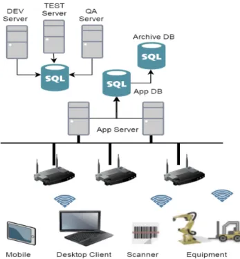
The summary of the integration in one figure is shown in Figure 1, while the schematic overview of the system architecture is shown in Figure1. The tools and devices used in realizing the use-case are listed below, for details see [34]:

• Siemens S7-1200 PLC

• KTP400 Touch Panel HMI

• Stepper Motor+Driver

• Baxter as a collaborative robot

• Conveyor belt

• Proximity sensor

• Solidworks to design the tester to be 3D printed

• Siemens TIA Portal V13 for PLC and HMI programming

• Robot Operation System (ROS) for programming the baxter cobot

• DELMIA Apriso MES solution

• SAP ERP solution

• Teamcenter PLM solution

B. TECHNICAL ASPECTS OF MES IMPLEMENTATION A typical MES hardware architecture is presented in Figure1. In the most demanding scenarios, a database tier be separated from the application and web tiers. In such an approach, it is possible to configure the database tier according to the database vendor-specific high availability configu- rations without impacting the MES software tiers. An example of such a deployment scenario can be achieved by clustering the database over the MSCS (Microsoft Cluster Service) cluster and the other tiers of the system according to the clustering and NLB (Network Load Balancing) approach. Such a configuration requires a minimum of six servers as this is suggested in Figure2.

FIGURE 1. Overview of the components used in the use-case.

The Database layer is responsible for storing data and is fail over managed by Windows Clustering Services or other database vendor specific technology. The Application layer is responsible for background processing and delivering data for Web Services and the Client. The Web Sever layer is responsible for server side user interface rendering and interfacing with other systems. The Client layer is responsible for client side UI rendering. In the most basic architecture MES solutions can work on a single server such approach is most commonly used for non-production environments where availability and performance constraints are low pri- ority. Typical MES deployment of production environments allows splitting every system tier into separate physical

(5)

FIGURE 2. Overview of the MES data bases.

FIGURE 3. Overview of a typical MES server network.

servers such as this is shown in Figure3. During the Build phase of the project the solution is developed and customized by the development team on a development server (DEV Server). Once a phase is completed, this is transferred to a TEST server. If the solution passes all the tests, has to be validated. In the most cases the validation of a solution is done in a QA (Quality Assurance) Server with dummy or real data from the production. After validation the whole solution is deployed to App Server which means live production.

III. DATA MINING METHODS

Both Root Cause Analysis (RCA) and prediction were aimed to be performed by employing data mining methods, in order to build an appropriate model for the given system. The model consists of:

• the target variables, which have to be predicted and against which the causal influence of the other features is analysed;

• the relevant features that influence each target variables;

• the probability distributions corresponding to the target variables, respectively of mathematical relations between each target variable and the other variables.

The formal description of this model is provided below:

M = {T,RF_T,V_RF}, where

T =F(Rf₁,Rf₂, . . . ,Rf_n), RFT = {Rf1,Rf2, . . . ,Rfn},

V_RF = {relevance,probability_distribution} (1) In (1),T represents a target variable, RF_T is the set of the relevant features that influenceT,Fis the mathematical formula through which the relation between the relevant features andT can be expressed,V_RF is the vector associated to each relevant feature, consisting of the relevance and probability distribution associated to this feature.

The following steps were taken into account in order to build this model: 1) Establish the target variables, which have to be predicted and against which the causal influence of the other features is analysed; 2) Apply feature selection methods, in order to determine the relevant features that influence each target variable; 3) Apply appropriate methods, in order to predict the values of the target variables as a function of the other variables, respectively to determine the probability distributions of the relevant features. 4) Validate the generated model through supervised classification.

A. FEATURE SELECTION METHODS

Concerning the data mining methods, the most appropriate high performance techniques were chosen, in order to perform RCA and prediction in optimum manner. In the context of the RCA phase, specific feature selection methods were firstly applied, in order to determine the most relevant features that influence the target variables (in this case the Endpoint Force and the Endpoint Torque). Among the existing feature selection methods, the Correlation based Feature Selection, the Consistency based Feature Subset Evaluation, respectively the Gain Ratio Attribute evaluation, which provided the best results in the former experiments, were chosen.

For the CFS technique, a merit was computed, with respect to the class parameter [21] and assigned to each feature group, as described by the formula (2).

Merits = kr_cf

p(k+k(k−1)r_ff) (2)

(6)

In (2)rcf represents the average correlation of the features to the class,rff is the average correlation between the features andkis the number of the elements in the subset.

The second technique which was employed tries to assign a consistency measure to each possible group of features and finally chooses the group with the highest consistency values.

The consistency is computed as indicated by the formula (3):

Consistency_s =1− PJ

i=0|D_i| − |M_i|

N (3)

In (3) J is the number of all the possible combinations for the attributes within the s subset,|D_i| is the number of appearances of the combination i for all the classes, while

|M_i|is the number of appearances of combinationiwithin the class where this combination appears the most often. Thus, the consistency of the attribute subset decreases, if the global number of appearances of that combination (subset) is greater than the number of appearances of this combination within the class where it appears the most often.

The above described methods were always used in conjunction with a search algorithm, such as genetic search, best first search and exhaustive search [26].

The third technique assessed the individual features by assigning them a gain ratio with respect to the class [21], as provided in (4).

GainR(A_i)= (H(C)−H(C|Ai))

H(A_i) (4)

In (4),H(C) is the entropy of the class parameter,H(C|A_i) is the entropy of the classC after observing the attributeA_i whileH(Ai)is the entropy of the attributeAi.

The final relevance score for each feature was obtained by computing the arithmetic mean of the individual relevance values provided by each method. Only those features that had a significant value for the final relevance score (above a threshold) were taken into account.

B. OTHER METHODS

Still in the context of Root Cause Analysis, but also touching the problem of prediction, Bayesian Belief Networks were adopted, for determining those features that influenced the class parameter, and also their probability distributions.

The Bayesian Belief Networks technique aims to identify influences between the features, by generating a dependency network, represented as a directed, acyclic graph (DAG).

In this graph, the nodes represent the features, while the edges stand for the causal influences between these features, having in association the values of the conditional probabilities.

Within this graph, every node X has a set of parents, P, respectively a set of children,C.

The probabilities of the nodes are computed based on complex inferences. The probability of a node, which is due to the other nodes within the network, is determined by using formula (5).

P(x|e)≈P(e_c|x)P(x|e_P) (5)

In (5),P(x|e) is the probability of the current node due to the other network nodes,P(e_c|x) is the probability of the children due to the current node, whileP(x|eP) is the probability of the current node, with respect to the corresponding parents.

Within a Bayesian Belief Network, to each node a probability distribution table is assigned, which indicates the specific intervals of values for that node, with respect to the values of the parents.

In order to analyse the relationships among the considered variables, various types of regression were employed: linear, quadratic, cubic, logarithmic, power, inverse [20]. The linear regression classifier was also used in the Weka environment, in order to establish the mathematical relationship between the target variable and the other variables [26].

C. SUPERVISED CLASSIFICATION TECHNIQUES 1) CLASSICAL(TRADITIONAL) TECHNIQUES

In order to assess the relevant features and the prediction ability of the model, the following supervised classification methods and classifier combination schemes, well known for their performance, were taken into account: Support Vector Machines (SVM), Random Forest (RF), Multilayer Percep- tron (MLP), the AdaBoost meta-classifier combined with the C4.5 technique for decision trees [22], and also the stacking technique for classifier combination [23]. For the MLP technique, multiple architectures were experimented and the best one was adopted. Stacking (stacked generalization) represents a classifier combination technique (an ensemble method) that allows combining multiple predictors, in the following manner: a simple supervised classifier, such as linear regression, is taken into account as a meta-classifier (combiner) and receives at its inputs the output values provided by other classification techniques (usually basic learners such as SVM, decision trees, Bayesian classifiers or neural networks). Although it appeared around the year 1990, this technique evolved into a ‘‘super-learner’’, allowing to automatically choose the most appropriate classifier combination [23].

2) DEEP LEARNING METHODS

The prediction performance of the deep learning classification techniques was assessed, as well. For this purpose, two powerful techniques, appropriate for the classification of the Baxter robot technical data, were taken into account.

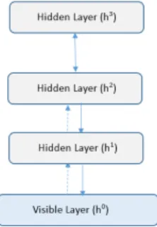
Thus, the Deep Belief Networks (DBN) and Stacked Denois- ing Autoencoders (SAE) classifiers, trained in supervised manner, were considered. TheDeep Belief Networks (DBN) constitute a complex technique, representing a class of deep neural networks, which is composed of multiple layers of latent variables, the so called ‘‘hidden units’’, having connections between the layers but not between the units within each layer, as shown in Figure4

In the current case, the DBN is based on Restricted Boltzmann Machines (RBM). RBM belongs to the category of Energy-Based Models (EBM), which associates a scalar

(7)

FIGURE 4. The architecture of a DBN.

energy to each distribution of the variables of interest. The corresponding learning process assumes to find the appropriate values of the parameters, so that the energy function has desirable properties, for example a minimum value. The Boltzmann Machines (BM) are a specific form of log-linear Markov Random Field (MRF), the corresponding energy function being linear in its’ free parameters. [24] Some of the variables are never observed, being hidden, so this method is able to represent complex distributions. RBMs restrict the BMs to those without visible-visible and hidden-hidden connections, having one layer of visible units and one layer of hidden units. RBMs can be stacked and trained using a greedy algorithm in order to achieve the Deep Belief Net- works (DBN). In this context, the hidden layers in Figure4 are represented by RBMs and each RBM (sub-network) hidden layer serves as the visible layer for the next. The joint distribution between the observed vectorsx, respectively the hidden layersh_k, is expressed in (6). [24]

P(x,h¹,h², ...,h^l)=(

l−2

Y

k=0

P(h^k|h^k+1))P(h^l−1,h^l)) (6)

In (6),x =h⁰,lis the number of the hidden layers of the DBN,P(h^k|h^k+1) is a conditional distribution for the visible units conditioned on the hidden units of the RBM at levelk andP(h^l,h^l−1) is the visible-hidden joint distribution within the top level RBM. In order to train a DBN in a supervised manner, a logistic regression layer must be added on the top of the network

The Stacked Denoising Autoencoder technique was also considered. An autoencoder usually takes an inputx∈[0;1]^d and first maps it, with the aid of an encoder, to a hidden representationy∈[0;1]^d⁰, through a deterministic mapping, as expressed by the formula (7):

y=s(Wx+b) (7)

In (7),sis a non-linear function, as, for example, the sigmoid, W is the weight matrix and b is a constant, chosen by the designer. The latent representation (code)y, can be mapped back intoz, a reconstruction of the same shape asx, using a similar transformation. The denoising auto-encoder is a stochastic version of the auto-encoder, which tries to encode the input, preserving the information concerning the input and

also tries to undo the effect of a corruption process applied to the input of the auto-encoder in a stochastic manner. The reconstruction error can be measured in many ways, the traditional squared errorL(xz) = ||x −z||², being an appropriate method for this task, in many situations. The codey can be considered a distributed representation, capturing the main factors of variation within the data, fact that makes this method similar to the Principal Component Analysis (PCA) technique. However, if the hidden layer is non-linear, the autoencoder captures more complex information regarding the main modes of variation within the data.

The Denoising Autoencoders can be stacked, resulting a Deep Autoencoder that uses the output of the autoencoder which is one layer below in order to feed the current layer.

An unsupervised pre-training is firstly performed, which assumes to train separately each layer, as a denoising autoencoder, by minimizing the reconstruction error of its input.

A second stage of supervised tuning can be performed, aiming to minimize the prediction error concerning a supervised task, by adding a logistic regression layer on the top of the network, so it will be trained as a Multilayer Perceptron [24].

3) CLASSIFICATION PERFORMANCE ASSESSMENT

In order to assess the classification performance, the following parameters were considered: the classification accuracy (recognition rate), the True Positive (TP) rate (sensitivity), the True Negative (TN) rate (specificity), the area under the ROC curve (AuC), respectively the Root Mean Squared Error (RMSE) [26]. The correlation was also taken into account in order to assess the prediction performance of the classifiers when considering the Endpoint Force, respectively the Endpoint Torque measured at the left and right limb of the robot as continuous target variables.

D. THE DATASET

The experimental dataset was gathered during the real- time activity of the Baxter robot, within the Baxter robot’s database and referred to collision events. An instance in this dataset consisted of the values of some significant parameters, such as the Endpoint Force and the Endpoint Torque, the five components of the Impact Torque and Squish Torque, as well as values of some control parameters, corresponding to the left and right limb of the robot, measured at a certain moment in time, the number of distinct attributes within the data being 50. According to the Baxter robot technical specifications [19], the impact torque corresponds to a sudden change in torque detected at one of the robot joints, associated to the to the situations when the moving robot arm meets, for example, a human. The squish torque appears when the moving robot arm tries to push a rigid stationary object, such as a wall. In this moment, the torque immediately increases above the threshold and the movement automatically stops, being resumed after two seconds.

At the end, a dataset of 992 instances, with no missing data, registered at a frequency of about 1 Hz, was achieved, which was employed in the further experiments.

(8)

IV. RESULTS A. DATA ANALYSIS

In order to detect subtle relations between the significant parameters of the Baxter robot, some experiments were firstly performed using Weka 3.7 (Waikato Environment for Knowledge Analysis) [26].

First, the Conjunctive Rule of Weka was applied on the whole dataset, in order to unveil subtle relationships that exist between the considered parameters. Then, feature selection methods were employed, in Weka 3.7, as well. The Corre- lation based Feature Selection (CfsSubsetEval) method and the Consistency Subset Evaluation (ConsistencySubsetEval) technique, both in combination with genetic search, as well as the Gain Ratio Attribute Evaluation technique in combination with the Ranker method, were considered. For each attribute, a relevance score was computed, corresponding to each method and the final score resulted as an arithmetic mean of the individual relevance scores. Concerning the CfsSub- setEvalandConsistencySubsetEvalmethods, the individual score assigned to the attribute was the score associated to the whole subset. Only those attributes having a final relevance score above a threshold (0.3), were taken into account. The type of dependency between the variables was analysed as well, using the Regression method within the IBM SPSS environment.

The Conjunctive Rule of the Weka 3.7 environment revealed the existence of a dependency between the endpoint Force and the endpoint Torque, as described in (8):

(f.endpointForce>4.109795)=>

f.endpointTorque=1.799236 (8)

Although the fact that the Endpoint Torque depends on the Endpoint Force is obvious from the definition of the torque parameter (which is the moment of force), the Conjunctive Rule of Weka suggests that if the Endpoint Force is greater than a threshold, then the Endpoint Torque should have a constant, maximum value (1.799). A similar relationship resulted when analyzing the data corresponding to the left limb of the robot.

Within the IBM SPSS environment [25], a linear and quadratic regression between the two above mentioned variables was also revealed, the R-Square coefficient being 0.999 in all these cases. The corresponding graphical representation is provided below, in Figure5.

In the further experiments, the Endpoint Torque and the Endpoint Force, measured at the left, respectively at the right limb of the Baxter robot, were taken into account as being the target variables.

First, the data was divided in two classes, according to the value of the Endpoint Torque parameter. For the right limb of the robot, if the Endpoint Torque value was below 1.75, the class assigned to the corresponding items was 1, otherwise the class 2 was assigned. For the left limb of the robot, the Endpoint Torque value which delimited the two considered classes was 1.62.

FIGURE 5. The existing correlations between the endpointForce and the endpointTorque parameters.

The feature selection methods were employed, as described above, in order to discover those features which influence the class parameter. Considering, as the target variable, the End- point Torque measured at the right limb of the robot, the most significant feature set is provided below, in (9).

RFSet1Right = {f.impactTorqueExpected₁, f.impactTorqueExpected3,

f.impactScalerInitial₁,f.accCmd₁, f.accCmd5,f.SquishTorque1,

f.SquishTorque5,f.endpointForce} (9) For the left limb of the Baxter robot, considering the Endpoint Torque as the target variable, the best set of relevant features is provided in (10):

RFSet1Left = {f.impactTorqueExpected₀, f.squishTorque2,

f.squishTorque3,

f.squishTorque₅,f.endpointForce} (10) It results that the Endpoint Force also influences the End- point Torque, the impactTorqueExpected, squishTorque and accCmd components being also relevant in this situation. The data was also split in two classes, according to the Endpoint Force parameter. Then, the feature selection techniques were applied within the Weka 3.7 environment. The following parameters resulted as directly influencing the Endpoint Force, considering the right limb of the robot, as depicted in (11):

RFSet2Right = {f.impactTorqueExpected₄,

f.impactTorqueExpected5,f.accCmd2, f.endpointTorque} (11) It results that the Endpoint Torque also influences the Endpoint Force, the impactTorqueExpected4, impactTorqueExpected5andaccCmd2parameters being also

(9)

relevant in this case. For the left limb of the robot, the best set of relevant features is provided in (12):

RFSet2Left

= {f.impactTorqueScaledSum, f.impactTorque₄,

f.impactTorqueExpected0,f.impactTorqueExpected1, f.impactTorqueExpected3,f.impactTorqueExpected5, f.impactTorqueScaled₃,f.impactScalerFinal₄, f.squishTorque2,f.squishTorque3,f.squishTorque4, f.squishTorque₅,f.endpointTorque} (12) One can notice again the importance of the endpoint Torque and of the Expected Impact Torque, but also of some components of the Squish Torque and of the final Impact Scaler.

Predictions:The LinearRegression classifier of Weka 3.7 was applied, in order to unveil linear relationships between the target variables and the other variables. After applying linear regression in Weka, considering the Endpoint Torque at the right limb of the robot as a target variable, the following relation resulted concerning the Baxter robot’s parameters, as presented in (13):

f.EndpointTorque

=0.0164∗f.impactTorque₅

+15.3446∗f.impactTorqueExpected2

+0.0276∗f.impactTorqueExpected₃ +(−0.0123)∗f.impactTorqueScaled0

+(−0.0445)∗f.impactTorqueScaled3

+(−0.0796)∗f.impactTorqueScaled₅ +(−0.1225)∗f.squishTorque0

+(−0.0959)∗f.squishTorque₁ +0.0856∗f.squishTorque4

+0.8362∗f.squishTorque₅

+0.3886∗f.endpointForce+2.5188. (13) Thus, the Endpoint Torque parameter depends heavily on the second component of the Expected Impact Torque value, on the zero, first, fourth and fifth components of the Squish Torque, on the Endpoint Force, but also on other components of the Expected Impact Torque, of the Squish Torque, respectively on the Scaled Impact Torque. For the left limb of the Baxter robot, a similar relationship, illustrated in (14), resulted after applying the LinearRegression classifier:

f.endpointTorque

= −0.217∗f.impactTorqueExpected0

+10.7676∗f.impactTorqueExpected₁ +143.8943∗f.impactTorqueExpected2

+0.7051∗f.impactTorqueExpected₃ +(−42.3351)∗f.impactTorqueExpected4

+6.2987∗f.impactTorqueExpected5

+0.9768∗f.impactTorqueScaled1

+4.0269∗f.impactTorqueScaled₅ +(−0.3214)∗f.squishTorque₀ +0.0979∗f.squishTorque1

+0.2161∗f.squishTorque₂ +0.1089∗f.squishTorque3

+0.2236∗f.squishTorque₄ +(−0.0768)∗f.squishTorque5

+0.3666∗f.endpointForce

+(−0.0801) (14)

The importance of the Endpoint Force parameter, of the expected Impact Torque (components 2, 3 and 4), of the scaled Impact Torque can be noticed again, but also the relevance of the squish torque (especially the components 0, 2, 3, and 4).

Then, the technique of Bayesian Belief Networks (BayesNet) with Bayesian Model Averaging (BMA) Estima- tor andK2search was applied [20].The target variable, in this case, was the Endpoint Torque, measured at the left limb of the Baxter robot. Among the most relevant parameters, detected through the technique of Bayesian Belief Networks, the Expected Impact Torque, the Squish Torque and the Endpoint Force were met. The probability distribution tables for component 5 of the Expected Impact Torque, respectively for components 2 and 5 of Squish Torque are provided within Table1, Table2, respectively Table3.

TABLE 1.Probability distribution Table:impactTorqueExpected₅.

TABLE 2.Probability distribution Table:SquishTorque₂.

TABLE 3.Probability distribution Table:SquishTorque₅.

From Table1it results that for low values of the 5^thcom- ponent of the Expected Impact Torque the Endpoint Torque has low values with a probability of 0.948 and high values with a probability of 0.916. For medium values of the fifth component of the Expected Impact Torque, the Endpoint Torque is more likely to have higher values, with a probability of 0.083, while for higher values of the fifth component of the Expected Impact Torque, the Endpoint Torque is more likely to take lower values, with a probability of 0.045.

(10)

From Table2it results that for low values of the component 2 of the Squish Torque parameter the Endpoint Torque takes lower values with a probability of 0.059 and higher values with a very small probability of 0.001, while for higher values of the second component of Squish Torque, the Endpoint Torque takes, more likely, higher values, with a probability of 0.999. It results that there is a direct dependency between the SquishTorque₂ parameter and the Endpoint Torque (while SquishTorque₂ increases, Endpoint Torque also increases).

From Table3it results that for low values of the component 5 of the Squish Torque parameter the Endpoint Torque is more likely to take lower values with a probability of 0.807, for medium values of the 5th component of the Squish Torque the Endpoint Torque takes, more likely, higher values, with a probability of 0.256, while for higher values of SquishTorque5the Endpoint Torque takes, more likely, higher values, with a probability of 0.309. Thus, there is a direct dependency between the SquishTorque₅ parameter and the Endpoint Torque (while SquishTorque5 increases, Endpoint Torque also increases).

B. CLASSIFICATION PERFORMANCE ASSESSMENT In order to assess, through classifiers, the possibility of prediction, but also to validate the part of the model consisting of the relevant features, traditional classification techniques, well known for their performances, such as the Support Vector Machines (SVM), Random Forest, Multilayer Per- ceptron (MLP), AdaBoost combined with the C4.5 decision trees based classifier, respectively the stacking combination scheme that took into account the above mentioned classifiers, were firstly experimented. The deep learning techniques described above, based on Deep Belief Networks (DBN), respectively Stacked Autoencoders (SAE) were also considered. The traditional classification techniques were implemented by using the Weka 3.7 library. For SVM, the John Platt’s Sequential Minimal Optimization (SMO) was employed, with normalized input data, respectively Radial Basis Function (RBF) or polynomial kernel, the corresponding configuration being tuned in order to achieve the best performance in each case. The RandomForest technique with 100 trees was adopted, as well. Concerning the MLP classifier, the MultilayerPerceptron method of Weka was implemented, with a learning rate of 0.2 and a momentum of 0.8, aiming to achieve both high accuracy and high speed of the learning process and also to avoid overtraining. Multiple architectures of MLP were experimented and the best one was finally taken into account, these being the following: the architecture with a single hidden layer and the number of nodes equal with the arithmetic mean between the number of attributes and the number of classes, denoted by a; the architecture with two hidden layers, with the same number of nodes in each layer, this being either a, or a/2; the architecture with three hidden layers, with the same number of nodes in each layer, this being either a, or a/3. The AdaBoostM1 technique with 100 iterations, standing for the

AdaBoost metaclassifier, was also implemented, in conjunction with the J48 method standing for the C4.5 algorithm.

The StackingC classifier combination scheme of Weka 3.7, standing for an improved version of the Stacking combination scheme, was experimented as well, using LinearRegression as a meta-classifier and the above mentioned basic learners, in an optimum combination, determined through experiments. All these classifiers were applied after performing feature selection. The 5-folds cross-validation strategy was adopted in all of these cases, in order to assess the classification performance, meaning that 4/5 of the data was used for training and 1/5 of the data was used for validation, this pro- cedure being repeated 5 times for different training/validation sets [20].

The deep learning methods were employed, as well, by using the Deep Learning Toolbox for Matlab [27], for comparison with the traditional methods, from the accuracy point of view. The corresponding parameters, such as the number of layers, the initial learning rate, the momentum, the batch size and the number of training epochs were fine tuned in order to achieve the best classification performance, in each case. In order to assess the classification performance, each of these methods was unfolded to a neural network having the same structure. In order to evaluate this classifier for supervised learning, an additional layer was added, having a number of output nodes equal with the number of classes (two, in this case). The whole data was split so that two-thirds of it was used for training, respectively one third of these data constituted the test set. The prediction was also performed by considering continuous attributes as target variables within the IBM SPSS Modeler environment [28].

In this case, the correlation metric was taken into account for prediction performance assessment.

1) CLASSIFICATION PERFORMANCE ASSESSMENT WHEN TAKING INTO ACCOUNT THE ENDPOINT TORQUE CORRESPONDING TO THE RIGHT LIMB OF THE ROBOT

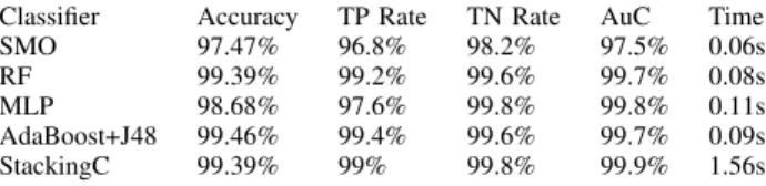
The values of the classification performance parameters obtained through traditional classification methods when taking into account the Endpoint Torque corresponding to the right limb of the robot are depicted within Table4. It results, from this table, that the Endpoint Torque corresponding to the right limb of the robot can be predicted with an accuracy bigger than 98%. However, the best accuracy, of 99.6%, as well as the highest value of the sensitivity, of 99.8% and

TABLE 4.Classification performance assessment for the prediction of the Endpoint Torque, for the right robot limb.

(11)

the highest value of the AuC, of 99.9%, were obtained in the case of the Stacking combination scheme that took into account all the others classifiers, without the MLP classification technique, which would have increased the processing time. The maximum value of the TN Rate, of 99.8%, was achieved for the RF classifier. Concerning the values of the sensitivity(TP Rate)or specificity(TN Rate), denoting, in this case, the probability to predict a lower, or a higher value of the Endpoint Torque, one can notice that they also were above 98% in all cases. Concerning the SMO classifier, the configuration that provided the best result in this case was that based on a polynomial kernel of 7th degree. For the MLP classifier, the configuration having a single hidden layer and a number of nodes equal with the arithmetic mean between the number of attributes and the number of classes provided the best results in this case.

2) CLASSIFICATION PERFORMANCE ASSESSMENT WHEN TAKING INTO ACCOUNT THE ENDPOINT TORQUE CORRESPONDING TO THE LEFT LIMB OF THE ROBOT The values for the classification performance parameters for the prediction of the Endpoint Torque at the left limb of the robot, through classical learners, are illustrated in Table 5.

It results that an accuracy above 96.5% was obtained in all cases, the highest value, of 99.89%, being achieved in the case of the StackingC combination scheme that employed as basic learners all the others classifier, without MLP. It can also be remarked that for the sensitivity(TP Rate)the highest value, of 98.2%, resulted both for AdaBoost combined with J48 and for the StackingC combination scheme, while for the specificity(TN Rate), the highest value, of 99.8%, was obtained in the case of the SMO classifier with a polynomial kernel of degree 7. The best value for the AuC parameter, of 99.9%, resulted in the case of the RF classifier and of the StackingC combination scheme. For the MLP classifier, the configuration with three hidden layers, having, within each layer, a number of nodes equal with the arithmetic mean between the number of attributes and the number of classes, led to the best results in this case. Concerning the SMO classifier, the configuration employing a polynomial kernel of degree five provided the best performance in the current situation.

TABLE 5. Classification performance assessment for the prediction of the Endpoint Torque, for the left robot limb.

3) CLASSIFICATION PERFORMANCE ASSESSMENT WHEN TAKING INTO ACCOUNT THE ENDPOINT FORCE

CORRESPONDING TO THE RIGHT LIMB OF THE ROBOT Regarding the case when the Endpoint Force at the right limb of the robot was taken into account as a target variable,

the classification performance parameters, assessed through traditional classification methods, are provided in Table6.

The maximum classification accuracy, of 99.46%, as well as the maximum sensitivity(TP Rate), of 99.4%, resulted in the case of the AdaBoost meta-classifier combined with the J48 method, the maximum specificity(TN Rate) of 99.8%

resulted for the MLP classifier and for the StackingC combination scheme involving all the classifiers, except MLP.

The highest value ofAuCof 99.9% resulted in the case of the StackingC combination scheme and for the RF classifier.

Concerning the MLP classifier, the architecture with two hidden layers, having, within each such layer, a number of nodes equal with the arithmetic mean between the number of attributes and the number of classes, led to the best performance. Referring to the SMO classifier, the configuration with a polynomial kernel of degree three provided the best performance in this case.

TABLE 6.Classification performance assessment for the prediction of the Endpoint Force, for the right robot limb.

4) CLASSIFICATION PERFORMANCE ASSESSMENT WHEN TAKING INTO ACCOUNT THE ENDPOINT TORQUE CORRESPONDING TO THE LEFT LIMB OF THE ROBOT The classification performance parameters, assessed through traditional classification techniques, corresponding to the case when the Endpoint Torque value was aimed to be predicted are depicted within Table7. In this case, the maximum accuracy, of 99.89%, the maximum specificity (TN Rate) of 99.9% and the maximumAuCof 99.9% were achieved for the AdaBoost meta-classifier combined with the J48 method and for the StackingC combination scheme that implemented all the others classifiers, except MLP, as basic learners. The highest sensitivity(TP Rate)of 99.98% resulted in the case of the AdaBoost classifier combination scheme. Regarding the MLP classifier, the architecture with one hidden layers, having a number of nodes equal with the arithmetic mean between the number of attributes and the number of classes, provided the best performance. Concerning to the SMO classifier, the configuration with a polynomial kernel of degree five yielded the best classification performance.

TABLE 7.Classification performance assessment for the prediction of the Endpoint Force, for the left robot limb.

(12)

V. DISCUSSIONS

As one can notice from the experiments described above, the target variables, the Endpoint Force and the Endpoint Torque, are influenced by the Squish Torque and Impact Torque parameters measured at the joints of the Baxter robot and also by other control parameters of the robot. It can be observed that, generally, when the values of the components of the Impact Torque and Squish Torque increase, the End- point Torque and Endpoint Force increase, as well. Also, the Endpoint Torque depends on the Endpoint Force, between these two variables existing various types of correlations (linear, quadratic).

The values of the Endpoint Torque and Endpoint Force can be predicted, through traditional classification techniques, as a function of the other variables (Squish Torque, Impact Torque and control variables), with an accuracy above 96%

in all cases.

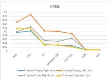
Figure 6illustrates a centralization concerning the accuracies of the predictions regarding the values of the End- point Torque and Endpoint Force parameters corresponding to the right limb, respectively to the left limb of the Baxter robot, due to the considered classifiers. The accuracies were measured this time through the Root Mean Squared Error (RMSE) parameter, the deep learning techniques being taken into account, as well, for comparison with the traditional methods. It can be noticed that, considering the available experimental data, the best accuracy values corresponded to the prediction of the Endpoint Torque at the right limb of the robot (the arithmetic mean of the recognition rates being above 99.4%, respectively the arithmetic mean of the RMSE values being 0.0437), followed by those corresponding to the prediction of the Endpoint Force at the left limb of the robot (the arithmetic mean of the recognition rates being above 99.2% , respectively the arithmetic mean of the RMSE values being 0.0467 in this case), then by the case when the Endpoint Force at the right limb of the robot was aimed to be predicted (the arithmetic mean of the recognition rates being above

FIGURE 6. The comparison of the RMSE values corresponding to the prediction of the Endpoint Force and Endpoint Torque at the left and right limb of the Baxter robot.

98.8% in this case, respectively the arithmetic mean of the RMSE values being 0.058) and finally by the case when the Endpoint Torque at the left limb of the robot was assessed (the arithmetic mean of the recognition rates being above 98.05%, while the arithmetic mean of the RMSE values was 0.092). Concerning the traditional classification techniques, the best classification performances, in both accuracy and time, were achieved for the StackingC combination scheme that implemented the SMO, RF and AdaBoost classification techniques as basic learners, followed by the AdaBoost combination scheme implemented in conjunction with the J48 method, respectively by the RF method, fact that confirms the efficiency of these ensemble classification techniques.

The AdaBoost technique was efficient from both time and accuracy points of view. According to Figure6, it is obvious that the considered Deep Learning methods (DBN and SAE) overpassed the performances of the traditional classification techniques, the RMSE parameter taking values less than 0.01 in all the cases. Thus, the arithmetic mean value of the RMSE parameters was 0.0060 in the case of the SAE technique, while in the case of DBN, it was 0.0067. In the case of the DBN method, the architecture that led to the best classification performances was that containing five or seven hidden units of RBM type, the initial learning rate being 0.2, the momentum being 0.8, the batch size being 150 and the number of the training epochs being tuned to 100. In the case of the SAE technique, the configuration corresponding to the best classification performance was that with two hidden units (of Autoencoder type), the initial learning rate of 0.2, the batch size of 120 and 100 training epochs.

Prediction by correlation, considering as target continuous variables, was performed within the IBM SPSS Modeler [28].

The following classifiers were taken into account: Random Forest (RF), Support Vector Machines (SVM), respectively the Multilayer Perceptron (MLP) classifier with a single hidden layer having the number of nodes equal with the number of input features. The values of the correlation metric obtained for each target variable (Endpoint Torque, respectively Endpoint Force, measured at the right, respectively left limb of the Baxter robot) were always above 0.98 in all the considered cases, fact that confirms the previously obtained results. The arithmetic means of the correlation values, resulted for each classifier, are depicted within Table8.

As in the previous case, when assessing the accuracies of the binary classifiers, the best correlation values, having the arithmetic mean of 0.997, were obtained for the Endpoint Torque measured at the right limb of the Baxter robot, respectively for the Endpoint Force measured at the left limb of the Baxter robot, followed by 0.991, obtained when predicting

TABLE 8.Prediction performance assessment considering continuous target variables, through the arithmetic mean of the correlations.

(13)

the Endpoint Force at the right limb of the robot, respectively 0.986, when predicting the Endpoint Torque at the left limb of the Baxter robot.

Based on the obtained results, the Endpoint Force and Endpoint Torque at the left and right limbs of the Baxter robot can be tuned to minimum values, for reduce the damages caused by collisions. Considering the fact that the prediction accuracy for these target variables was always above 96%, it results that the tuning process will have an important impact concerning the efficiency and safety of the Baxter robot, mainly during the MOL phase of the corresponding PLM, facilitating the vertical integration of this equipment in the context of the MES of the company.

When comparing the results presented above with the state of the art achievements, it results that the accuracy obtained in the above described experiments is within the range, even better than the highest accuracy values corresponding to these achievements. This fact is illustrated within Table9.

TABLE 9. Comparison with the state of the art results.

A. PRACTICAL APPLICATIONS OF THE DATA MINING METHODS

In order to monitor the behaviour of the Baxter robot over time, some useful plots and 3D histograms will be automatically generated, according to the data-mining results described above, using Python or Matlab [29] development environments, which have interfaces with the Baxter robot [19]. Some eloquent examples of such plots and histograms, generated using the Matlab 2017 environment, are illustrated within the next figures.

Thus, Figure 7 provides a 2D plot, representing the Endpoint Force parameter as a function of the component 5 of to the Squish Torque parameter. According to this representation, the Endpoint Force parameter is, on average, increased when the Squish Torque 5 parameter takes negative values between−0.25 and−0.1, respectively when it takes positive values between 0.1 and 0.15.

The next figure, Figure 8, illustrates a 3D plot, representing the Endpoint Torque parameter as a function of 2nd and 5th components of the Squish Torque. Regarding the representation provided in Figure8, the color is proportional with the surface height. From Figure8it can be noticed that for low values of the 2nd and 5th components of the Squish Torque parameter, the Endpoint Torque has, on average, low values, while for medium and increased values of the 2nd and 5th components of Squish Torque, the Endpoint Torque can take both medium and increased values.

Figures 9, 10 and 11 represent 3D histograms, as follows:

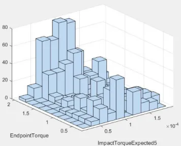
• Figure 9 illustrates the histogram of the variables Expected Impact Torque (the 5th component),

FIGURE 7. The plot of the Endpoint Force and a function of squishTorque₅.

FIGURE 8. The 3D plot of the Endpoint Force and a function of squishTorque₂andsquishTorque₅.

FIGURE 9. The 3D histogram of the variablesexpectedImpactTorque₅and endpoint torque.

respectively the Endpoint Torque. It can be noticed that for medium values of the 5th component of the Expected Impact Torque, often medium and high values of the

(14)

FIGURE 10. The 3D histogram of the variablessquishTorque₅and Endpoint Torque.

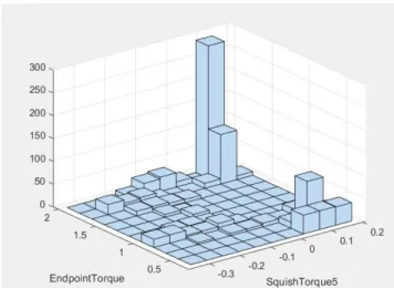
FIGURE 11. The 3D histogram of the variablessquishTorque₂and Endpoint Torque.

Endpoint Torque parameter are met, while for smaller values of the 5th component of the Expected Impact Torque, both small and higher values of the Endpoint Torque parameter are met.

• Figure10depicts the histogram of the parameters Squish Torque 5 and Endpoint Torque. One can remark that for increasing values of the 5th component of Squish Torque, high values of the Endpoint Torque are met mostly often, but small values of the Endpoint Torque can be met as well.

• Figure11depicts the histogram of the parameters Squish Torque, 2nd component, respectively Endpoint Torque.

It results that for small negative values of the 2nd component of Squish Torque increased values for the Endpoint Torque are often met, while for values of the 2nd component of Squish Torque which are around and above zero, small values of the Endpoint Torque parameter occur.

For Figure 9, 10and11, the vertical axis stands for the number of items having certain values of the parameters

represented on the other axes. The observations above confirm and complete the results provided within Tables1,2and3.

VI. CONCLUSIONS

As it results from the experiments, the data mining methods are able to unveil subtle relationships between the Baxter robot parameters. Thus, the Endpoint Force and the Endpoint Torque depend on each other and also on the Impact Torque and Squish Torque components, which are measured at the joints of the robot, so they and can be predicted on the basis of these values, with an accuracy above 96%. According to these experiments, plots expressing the relationships between these parameters can be dynamically represented to the user con- sole of the robot. Thus, the performances of the Baxter robot in the PLM context can be considerably improved. By tuning the Endpoint Force and Endpoint Torque at minimum values, the collision impact can be considerably reduced, fact that will have an important influence concerning the safety of this equipment facilitating the vertical integration process.

Concerning the future research, the aim will be to apply other advanced data mining methods, as well, such as association rules [31], clustering (grouping) techniques, in order to automatically divide the data in multiple classes [20], optimization techniques, such as Particle Swarm Optimization (PSO) [32], as well as to experiment more dimensionality reduction methods, before the classification phase.

ACKNOWLEDGMENT

The authors would like to thank to their company side colleagues (Laszlo Tofalvi, Levente Bagoly, Peter Mago) and colleagues from TUCN (Cristian Militaru, Mezei Ady Daniel, Mircea Murar) for their support realizing this work.

REFERENCES

[1] K. Jung, S. Choi, B. Kulvatunyou, H. Cho, and K. C. Morris, ‘‘A reference activity model for smart factory design and improvement,’’Prod. Planning Control, vol. 28, no. 2, pp. 108–122, 2017.

[2] H. S. Kanget al., ‘‘Smart manufacturing: Past research, present findings, and future directions,’’Int. J. Precis. Eng. Manuf.-Green Technol., vol. 3, no. 1, pp. 111–128, 2016.

[3] L. Monostori, ‘‘Cyber-physical production systems: Roots, expectations and R&D challenges,’’Procedia CIRP, vol. 17, pp. 9–13, Apr. 2014.

[4] R. Kohavi, ‘‘Data mining and visualization,’’ inProc. 6th Annu. Symp.

Frontiers Eng., 2001, pp. 30–40.

[5] J. Raphael, E. Schneider, S. Parsons, and E. I. Sklar, ‘‘Behaviour mining for collision avoidance in multi-robot systems,’’ inProc. Int. Conf. Auton.

Agents Multi-Agent Syst., 2014, pp. 1445–1446.

[6] R. Chuchra and R. Kaur, ‘‘Human robotics interaction with data mining techniques,’’Int. J. Emerg. Technol. Adv. Eng., vol. 3, no. 2, pp. 99–101, 2015.

[7] J. Li, F. Tao, Y. Cheng, and L. Zhao, ‘‘Big data in product lifecycle management,’’Int. J. Adv. Manuf. Technol., vol. 81, nos. 1–4, pp. 667–684, 2015.

[8] A. H. C. Ng, S. Bandaru, and M. Frantzén, ‘‘Innovative design and analysis of production systems by multi-objective optimization and data mining,’’ inProc. 26th CIRP Design Conf., vol. 50, 2016, pp. 665–671.

[9] C. Gröger, F. Niedermann, and B. Mitschang, ‘‘Data mining-driven manufacturing process optimization,’’ in Proc. World Congr. Eng. (WCE), London, U.K., vol. 3, Jul. 2012, pp. 1–7.