Chemical Engineering Journal 419 (2021) 129947
Available online 24 April 2021
1385-8947/© 2021 The Author(s). Published by Elsevier B.V. This is an open access article under the CC BY license (http://creativecommons.org/licenses/by/4.0/).
Dynamic flowsheet model development and digital design of continuous pharmaceutical manufacturing with dissolution modeling of the
final product
Brigitta Nagy
a,b, Botond Szil ´ agyi
c,*, Andr ´ as Domokos
a, Blanka V ´ eszi
a, Korn ´ elia Tacsi
a, Zsolt Rapi
a, Hajnalka Pataki
a, Gy ¨ orgy Marosi
a, Zolt ´ an K. Nagy
b,*, Zsombor Krist ´ of Nagy
aaDepartment of Organic Chemistry and Technology, Budapest University of Technology and Economics, H-1111 Budapest, Hungary
bDavidson School of Chemical Engineering, Purdue University, West Lafayette, IN 47907, USA
cFaculty of Chemical Technology and Biotechnology, Budapest University of Technology and Economics, H-1111 Budapest, Hungary
A R T I C L E I N F O Keywords:
Dynamic flowsheet modeling Integrated continuous manufacturing Dissolution modeling
Sensitivity analysis Optimization
A B S T R A C T
The integration of continuous unit operations imposes a challenge on the pharmaceutical companies aspiring to achieve plant-wide continuous manufacturing due to the additional complexity of the dynamic interactions, process control and quality assurance. To overcome this challenge, flowsheet modeling emerged as a viable tool to gain deeper process knowledge. In this work, the dynamic model of the integrated continuous manufacturing of acetylsalicylic acid (ASA) was formed based on real continuous unit operations. Furthermore, the surrogate model of the in vitro dissolution test of ASA capsules was integrated into the flowsheet model the first time to analyze the integrated manufacturing in light of the dissolution specifications of an immediate-release formu- lation. Systematic optimization studies were performed on the integrated process and on the continuous unit operations step-by-step, which clearly revealed the impact of the plant-wide dynamic modeling, as the integrated approach resulted in the threefold increase in the overall productivity and the parallel decrease in the required reactant excess. Sensitivity analyses of the operating conditions and the kinetic parameters were also performed.
The crystallization temperature emerged as one of the most critical parameters, which variation could even result in the failure of the dissolution specification. Moreover, by calculating the time-varying sensitivity indices, the dynamics of the error propagation could be studied. These results could facilitate the integration of existing continuous units, the development of the control strategy, and encourage the implementation of dissolution surrogate models into process flowsheet simulations.
1. Introduction
In the last decade, the pharmaceutical industry has started to un- dergo a vast transformation, which aims the implementation of flexible and efficient manufacturing as opposed to the traditional, conservative approach of fixed process conditions. This is promoted by several ad- vances in parallel. From the technology point of view, innovations in continuous manufacturing equipment are rapidly emerging, providing options for consistent and economical production [1], and the regula- tory agencies support the concept by providing guidelines [2] and ini- tiatives, such the Quality-by-Design (QbD) [3] and Process Analytical Technology (PAT) [4]. These principles focus on the knowledge- and
risk-based operation of the manufacturing process by the thorough mapping of the underlying critical material attributes (CMAs) and pro- cess parameters (CPPs) and their effect on the target product profile. The most important tools for this are real-time, in-line measurements as well as various statistical and mechanistic modeling methodologies [5,6].
Due to the additional complexity of continuous manufacturing lines, the importance of the systematic model-based design of the product and processes has increased. Mechanistic dynamic flowsheet models have been identified as excellent tools for representing the process knowledge and dynamically analyze the input–output relationship [7]. Together with widely used analysis tools, e.g., sensitivity analysis [8], this con- tributes to the identification of the excessive variation and risk of error propagation, the optimization of the process, and the development of
* Corresponding authors: Davidson School of Chemical Engineering, Purdue University, West Lafayette, IN 47907, USA (Z.K. Nagy); Department of Organic Chemistry and Technology, Budapest University of Technology and Economics, H-1111 Budapest, Hungary (B. Szilagyi)
E-mail addresses: szilagyi.botond@vbk.bme.hu (B. Szil´agyi), zknagy@purdue.edu (Z.K. Nagy).
Contents lists available at ScienceDirect
Chemical Engineering Journal
journal homepage: www.elsevier.com/locate/cej
https://doi.org/10.1016/j.cej.2021.129947
Received 10 December 2020; Received in revised form 16 March 2021; Accepted 17 April 2021
control strategies [7,9]. Furthermore, when continuous communication is enabled between the model and the real process, a digital twin is created, which can be further used e.g., for model-predictive control [10].
The concept of flowsheet modeling of continuous manufacturing has been already utilized by several authors for both the upstream (active pharmaceutical ingredient (API) manufacturing) and downstream (final product manufacturing) process steps, and software packages are also available to facilitate their development, such as gPROMS by Process Systems Enterprise [11]. As for the upstream part, a dynamic flowsheet model of ibuprofen synthesis and crystallization was developed and the uncertainty of the process was systematically studied [12]. Diab et al.
studied the flowsheet model of the synthesis and crystallization of rufinamide [13] and nevirapine [14] in the view of techno-economic considerations, such as minimizing the production costs. Most recently, Icten et al. published a three-part series of papers [15–17]
dealing with the development of a virtual plant for continuous manufacturing of carfilzomib intermediate, intending to gain a
mechanistic understanding of the synthesis, crystallization and filtration unit operations, and to use the modeling framework to identify the CPPs that impact the conversion in their integrated system.
From the perspective of the downstream process modeling of solid products, mainly the continuous feeding, blending and tablet compres- sion steps are integrated [18–20], but there are also examples for incorporating dry [21] and wet granulation [22] steps. Wang et al. [20]
utilized the developed flowsheet model for the optimization of the process to minimize the total cost of the manufacturing. In most of the studies [18–20,22] sensitivity analysis was performed using the unit operation parameters (e.g., residence times, flow rates) and final prop- erties of the product, e.g., tablet hardness and weight, API concentration as examined response variables. However, only a few modeling studies incorporated both the upstream and downstream manufacturing steps.
Sen et al. [23,24] used such a model for analyzing the mixing properties in connection with the crystallization, filtration and drying processes, while in another study [25] the simulations were used to improve the overall productivity and quality of the manufacturing. Moreover, no List of notations
Ai Pre-exponential factor of the ith reaction AS Antisolvent- solvent volume ratio B Nucleation rate [# m-3s−1] b Nucleation rate exponent [-]
c Concentration in solution [M] (in synthesis); [kgm−3] (in crystallization)
cd Mass fraction of API in the dissolution medium [-]
c*c Equilibrium solubility in the crystallization [kgm−3] c*d Equilibrium solubility in the dissolution medium [g ASA/ g
solution]
ci Impurity concentration [M] (in the synthesis); [kgm−3] (in crystallization)
cin Inlet concentration of solution [kgm−3]
cnorm Normalized concentration in solution [M] (in synthesis);
[kgm−3] (in crystallization) cs Solid concentration [kgm−3] D Dissolution rate [ms−1] DR Dissolved ratio [%]
d Dissolution rate exponent [-]
E(t) Residence time distribution EE Elementary effect
Ea,g Growth activation energy [Jmol−1]
Ea,i Activation energy of the ith reaction [Jmol−1] F Flow rate [m3s−1]
G Growth rate [ms−1] KL Langmuir constant [kgm−3]
kb Nucleation rate coefficient [# m−3 s−1] kd Dissolution rate coefficient [m s−1] kg Growth rate coefficient [ms−1]
ki Reaction rate constant of the ith reaction [Jmol−1] kv Volume shape factor [-]
L Linear size of crystals [m]
Ln Nuclei size [m]
mc Sample mass in the dissolution test [kg]
N Reactor number [#]
n Population density [# m−4] nin Initial population density [#m−43]
nMSE Normalized mean square error [M2]
nMSEnorm Normalized mean square error calculated for normalized concentrations [M2]
O(D) Objective function P Purity [%]
pi Coefficients of size-dependent dissolution [-]
R Universal gas constant, 8.314 JK-1mol−1 ri Rate law equation of the the ith reaction T Temperature [◦C]
t Time [s]
V Volume [m3]
v Antisolvent volume fraction in feed [-]
vc Crystal volume fraction in the dissolution medium [-]
X Conversion [%]
Greek Letters
α Effectiveness factor [-]
δ Dirac-delta function
μ2 2nd moment of the CSD [m2m−3] μ3 3rd moment of the CSD [m3m−3] μM Mean of elementary effects ρc Crystal density [kgm−3]
ρd Density of the dissolution medium [kgm−3] σ Relative supersaturation [-]
σ2 Standard deviation of the reactor residence time distribution [s]
σ2M Standard deviation of elementary effects τ Mean residence time [s]
Subscripts
a Acetylation c Crystallization d Dissolution j Sample point m Measured data
q Quenching
X Component in the reaction mixture 0 Initial state
studies were found where the final quality of the formulation was assessed from the point of dissolution properties, although the in vitro dissolution is one of the most important and routinely analyzed quality attributes of solid pharmaceutical products [26]. Hence, the mathe- matical description could significantly contribute to the product and process development and release testing. This could be achieved either by first principles-based or black-box modeling approaches [27].
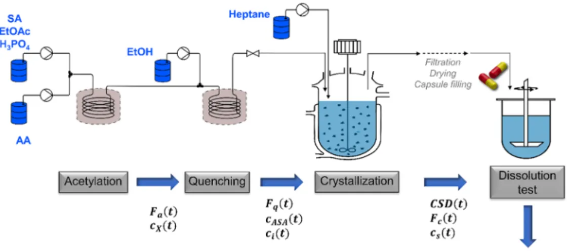
This paper presents the dynamic, integrated flowsheet model development for the continuous manufacturing of acetylsalicylic acid (ASA), involving a two-step flow synthesis and crystallization. The model was built to simulate the real continuous processes developed formerly by the authors of this paper [28,29]. In these former works, the unit operations were studied separately to analyze the effect of the different process parameters. As for the synthesis, the reaction mixture composition, processing temperature and residence times were opti- mized experimentally for maximal conversion and purity and minimal processing time [28], but the main priority was to obtain a reaction mixture which is directly connectable with electrospinning. The pro- cessing of this flow reaction mixture in continuous combined cooling and antisolvent crystallization process was also developed, where the effect of the crystallization temperature, the solvent system composition and residence time was studied on the crystal size distribution (CSD), yield and purity [29]. However, the integration of the synthesis and crystallization steps has not been achieved, yet. Therefore, to facilitate the integration of the existing unit operations, this work aimed the development of a dynamic flowsheet model to gain process under- standing on the operation of the continuous, integrated process. This study is also the extension of a previous publication [30], where the dynamic model of the continuous crystallization was presented, but it dealt mainly with the integrated simulation of the continuous crystal- lization and filtration, e.g., the effect on the CSD and solid concentration was analyzed on the continuous filtration. Consequently, together with the present work, the dynamic model of the fully continuous, integrated upstream process is achieved. The true potential of the integrated flowsheet model is demonstrated via optimization studies and sensitivity analysis. Furthermore, the surrogate in vitro dissolution model of cap- sules containing the obtained ASA powder is developed and integrated into the flowsheet model. Such a model can be useful when the disso- lution of the capsules is affected solely by the API characteristics.
Moreover, it could contribute to a better understanding of the CSD as CMA and the corresponding optimization and risk analysis of the API manufacturing process during the early stage of the drug development even in the case of more complex formulations. To the best of the au- thors’ knowledge, this is the first time when flowsheet modeling is uti- lized for studying the dissolution properties of the final product of continuous pharmaceutical manufacturing.
2. Materials and methods
2.1. Experimental procedures
The mathematical model of the integrated continuous synthesis- crystallization process and the in vitro dissolution properties was developed based on real, laboratory-scale continuous processes and experimental data. The synthesis and crystallization procedures have been originally published in [28] and [29] and the experiments used for the parameter estimation and validation of the synthesis and crystalli- zation steps came from these works. Although the experiments were originally conducted for the experimental development of the technol- ogies and not for the purpose of the mathematical model fitting, they were found to be suitable for the parameter estimations as the viable ranges of the operating conditions were explored in different combina- tions. The experiments were divided into calibration and validation sets.
A quasi-random division was aimed: the ratio depended on the total number of the available experiments, and the validation experiments were selected randomly, but it was also accounted that the validation set
should cover the whole range of the settings.
2.1.1. Synthesis
The modeling of the continuous synthesis of ASA was based on the experimental work of Balogh et al. [28]. The two-step flow synthesis consisted of acetylation and a subsequent quenching step. For acetyla- tion, a 1 mol L-1 solution of salicylic acid (SA) was prepared in ethyl acetate (EtOAc), also containing phosphoric acid (H3PO4) as a catalyst in 0.1 mol equivalent relative to SA. SA was acetylated continuously with excess acetic anhydride (AA). In the subsequent quenching step ethanol (EtOH) was added to the reaction mixture of the first step, to remove the excess AA and the quenchable impurities. The reactions were carried out in 8.77 and 1.83 m long tube flow reactors for the acetylation and quenching step, respectively with an inner diameter of 0.787 mm. 4 bar was used to maintain constant fluid flow conditions.
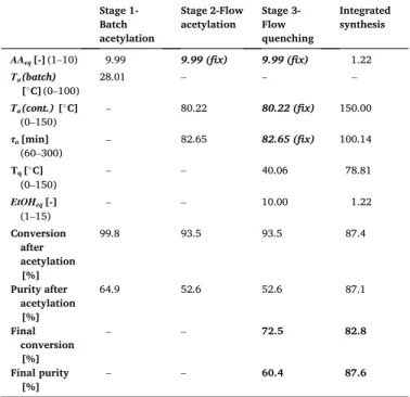
Acetylation experiments were conducted first in batch mode to analyze the effect of the AA excess (AAeq, mole equivalent relative to SA) and the acetylation temperature (Ta), then in continuous mode to adjust the temperature and the residence time (τa), while AAeq was fixed to 5, based on the outcomes of the batch experiments. At the quenching step, the EtOH ratio (EtOHeq, mole equivalent relative to the initial SA), residence time (τq), and quenching temperature (Tq), were analyzed in continuous mode, whereas AAeq, Ta and τa were fixed to 5, 55 ◦C and 180 min, respectively. The composition of the reaction mixture was measured by HPLC [28] every 10–20 min in the case of the batch acetylation and in the steady state of the continuous runs. Tables 1 and 2 summarize the acetylation and quenching experimental settings utilized in this study to estimate the kinetic parameters of the mathematical model. For further details on the experimental setup, the reader is referred to [28].
2.1.2. Crystallization
A combined cooling and antisolvent (CCAS) continuous crystalliza- tion method has been developed to crystallize the ASA from the reaction mixture obtained in the flow synthesis [29]. The crystallization experi- ments were performed in mixed-suspension, mixed-product-removal (MSMPR) continuous crystallizer operated at 235 mL constant volume and using heptane as antisolvent. Experiments were performed with 0.8 antisolvent volume fraction (v) and varying flow rates (Fc), temperatures (Tc) and residence times (τc) in the ranges of 5–20 mL min−1, 2–25 ◦C and 10–50 min, respectively. Details on the crystallization experimental setup, procedure, the experiments for the kinetic parameter estimation and the parameter estimation can be found in our previous publications [29,30].
2.1.3. In vitro dissolution testing
To investigate the effect of the crystal size distribution (CSD) on the in vitro dissolution of the final product (e.g., capsule), samples for dissolution testing were prepared by sieving ASA powder using 63, 100, Table 1
Experimental setting used for the kinetic parameter estimation and validation of the acetylation step.
Experiment
No. Ta[◦C] AAeq[-] Experiment
No. Ta[◦C] τa[min]
Abatch 1 20 1.5 Acont. 1 50 60
Abatch 2 20 5 Acont. 2 50 120
Abatch 3 50 1.5 Acont. 3 70 120
Abatch 4 50 10 Acont. 4 60 90
Abatch 5 77 5 Acont. 5 65 180
Abatch 6 77 10 Acont. 6 45 120
Abatch Val 1 20 10 Acont. 7 65 120
Abatch Val 2 50 5 Acont. 8 55 150
Abatch Val 3 77 1.5 Acont. 9 55 180
Acont. Val 1 70 60
Acont. Val 2 60 90
Acont. Val 3 45 180
150, 200, 300 and 500 μm sieve openings as well as by combining equal weights of sieve fractions (Table 3). Additionally, two continuously crystallized crystal products (MSMPR 1 and 2) were also used for vali- dation. The CSD of each sample was collected by a Parsum IPP 70-s inline particle sizing probe (Malvern Panalytical Ltd., UK) in batch mode. The samples were dispersed into the instrument for estimating the cord length of the crystals, which were used to construct the number- based CSDs in the 50–2000 μm size range with a logarithmic grid with 50 bins.
Then dissolution tests of 100 mg powders were carried out in powder form as well as in some cases (see Table 3) filling them into capsules. The tests were performed in a Hanson SR8-Plus dissolution tester (Hanson Research, USA) using the paddle method (United States Pharmacopoeia II). In the case of the capsules, a spiral capsule sinker was used to prevent the floating of the capsules. 900 mL of 0.1 N HCl solution was used as dissolution medium, stirred at 100 rpm and kept at constant tempera- ture of 37 ±0.5 ◦C, which ensured sink condition. An on-line coupled Agilent 8453 UV–VIS spectrophotometer (Hewlett-Packard, USA) was used to measure the concentration of dissolved ASA for 2 h by sampling every 2.5 min until 20 min, followed by sampling in every 10 min until 120 min.
Due to the possible degradation of the dissolved ASA to SA during the dissolution process (in preliminary tests ~ 2% of the ASA degraded in 1 h), the SA and ASA needed to be quantified simultaneously. Although this would be possible by an HPLC method, a Partial Least Squares (PLS) calibration model was developed for the evaluation of the UV–VIS spectra based on HPLC data to avoid the lengthy and labor-intensive HPLC measurement. The degradation was observed in the UV–VIS spectra by the gradual shift of the 229 nm ASA band, the appearance of a weak and broad SA band in the 270–320 nm region, which overlapped with a weak signal of the ASA in the 260–280 nm region. Therefore, the PLS model was developed for the 278–320 nm region of the mean-
centered UV absorbance spectra with 2 latent variables. The calibra- tion samples contained different amounts of ASA and SA in the 80–120 and 0–30 mg L-1 concentration ranges, respectively, which composition was determined by an HPLC method [28]. The R2 of the calibration and cross-validation was both 0.98, while a root mean square error of cali- bration and cross-validation of 4.78 and 5.46 mg L-1 was obtained, respectively.
2.2. Mathematical modeling and kinetic parameter identification The model-equations were solved in MATLAB R2020a (Math- Works®, USA), the integrated flowsheet simulation was implemented in Simulink 10.1 (MathWorks®, USA).
2.2.1. Flow synthesis
Based on the experimental observations [28], the reaction network of the acetylation step was constructed by accounting not only the conversion of SA to ASA (Eq. (1.a)) but also the formation of two im- purities, namely acetylsalicylic ethanoic anhydride (Impurity A) and acetylsalicylic anhydride (Impurity B) [28] (Eqs. (1.b) -(1.d)).
SA+AA→k1ASA+HA (1.a)
ASA+AA→k2A+HA (1.b)
A+ASAk⇌3,k3rB+HA (1.c)
SA+2AA→k4A+2HA (1.d)
where HA, A and B denote acetic acid, Impurity A and Impurity B, respectively.
At the subsequent quenching step, it was observed, that besides the decomposition of AA using EtOH, possible reactions of Impurity A and ASA also have to be considered (Eqs. (2.a) -(2.c)):
A+EtOH→k5ASA+EtOAc (2.a)
AA+EtOH→k6EtOAc+HA (2.b)
ASA+EtOHk⇌7,k7rSA+EtOAc (2.c)
In Eqs. (1)-(2) ki corresponds to the reaction rate constant expressed as
ki=Ai⋅e−Ea,iRT (3)
where Ai is the pre-exponential factor, Ea,i [J mol−1] is the activation energy, T [◦C] is the reaction temperature and R is the gas constant (8.314 J K−1 mol−1) of the ith reaction.
The rate law equations were expressed as ri=ki⋅∏
cX(t) (4)
Table 2
Experimental setting used for the kinetic parameter estimation and validation of the quenching step.
Experiment No. Tq[◦C] τq[min] EtOHeq[-] Experiment No. Tq[◦C] τq[min] EtOHeq[-]
Q 1 80 15 3 Q 11 80 21 3
Q 2 80 5 6 Q 12 90 26 3
Q 3 60 15 6 Q 13 100 31 3
Q 4 60 15 3 Q Val 1 80 15 6
Q 5 60 5 6 Q Val 2 80 5 3
Q 6 70 10 4.5 Q Val 3 60 5 3
Q 7 85 22 3 Q Val 4 70 10 4.5
Q 8 95 29.5 3 Q Val 5 90 26 3
Q 9 100 33 3 Q Val 6 100 21 3
Q 10 80 31 3
Table 3
Calibration and validation samples of the in vitro dissolution studies. The sam- ples that were measured both in powder and capsule form are indicated in bold.
Calibration samples Validation samples
Sample
name Sieve fraction [μm] Sample
name Sieve fraction [μm]
63 63–100 63 þ300 (63–100) þ(300–500)
100 100–150 63 þ100 þ
150 (63–100) þ(100–150) þ(150–200)
150 150–200 63 +200 +
500 (63–100) +(200–300)+ (>500)
200 200–300 0 +63 (<63)+(63–100)
300 300–500 100 100–150
500 >500 150 150–200
100 þ300 (100–150)
þ(300–500) 200 200–300
150 þ200 (150–200)
þ(200–300) 300 300–500
200 þ300
þ500 (200–300)
þ(300–500) þ(>500) MSMPR 1 – 63 þ500 (63–100) þ(>500) MSMPR 2 –
where cX denotes the concentration of the reaction component taking part in the given reaction. The rate law equations for each reaction are detailed in the Appendix.
The continuous flow synthesis can be described using an axial dispersion tubular reactor model, which consists of a set of partial dif- ferential equations (PDEs) [31]:
∂cX
∂t = − vx⋅∂cX
∂x +Dm⋅∂2cX
∂x2 +r (5)
where x corresponds to the spatial coordinate along the flow reactor, t is the time, cX is the concentration of the reaction component X, Dm is dispersion coefficient and r represents a set of rate law equations. The initial conditions for the PDEs correspond to the initial concentrations along the length of the reactor. At the reactor inlet and outlet, the Danckwerts boundary conditions apply [31], where the inlet boundary conditions are
vx⋅[cX(0) − cX0] − Dm⋅dcX
dx
⃒⃒
⃒⃒
x=0
=0 (6)
and the outlet boundary conditions are given as:
dcX
dx
⃒⃒
⃒⃒
x=L
=0 (7)
Although Eqs. (5)-(7) enables the concentration calculation through time and the spatial coordinate of the reactor, it requires the solution of PDEs, which cannot be directly implemented in the integrated, dynamic flowsheet simulation in Simulink. To overcome this problem, a tank-in- series (TIS) approximation of the axial dispersion model was used in this study, approximating the tubular flow reactor as a cascade of N equal- sized continuous stirred-tank reactors (CSTRs). In this case, assuming constant working volume, an ordinary differential equation (ODE) sys- tem was formed for each CSTR to describe the changes in the concen- trations of the reaction components for both the acetylation (Eq.8) and quenching (Eq.9) steps. (See the Appendix for the complete ODE systems.)
dca,X
dt =r+c0a,X− ca,X
τa (8)
dcq,X
dt =r+c0q,X− cq,X
τa (9)
In Eqs. (8)-(9), the subscripts a and q are referring to the acetylation and quenching step, respectively, τ denotes the mean residence time [s]
in the reactor, which is infinite during the modeling of the batch re- actions and expressed as Eq. (10) for the continuous reactor.
τ=V
F (10)
where V is the reactor volume [m3] and F is the flow rate [m3 s−1].
For Eqs. (8)-(9), the initial conditions ca,X(0) =ca,X,0 and cq,X(0) =cq,X,0
apply, where the initial ca,X,0 concentration was calculated based on the concentration of the SA solution and the applied AAeq, while cq,X,0 was calculated from the outlet acetylation concentrations and EtOHeq.
The volume of the CSTRs in the cascade (Vi) is calculated by dividing the total volume of the flow reactor by the reactor number N (Eq. (11)).
Vi=V
N (11)
The number of the necessary reactors was derived based on the reactor residence time distribution (RTD). The reactors were assumed to operate as laminar flow reactors (the Reynolds numbers ranged from 0.5 to 5 for the reactor settings summarized in Table 1-2), which residence time is expressed as Eq. (12) [31].
E(t) =
⎧⎪
⎨
⎪⎩ 0if t<τ
2 τ2 2t3if t≥τ
2
(12)
where the mean residence time (τ) and the standard deviation (σ2)of the RTD is calculated as:
τ=
∫∞
0
tE(t)dt (13)
σ2=
∫∞
0
(t− τ)2E(t)dt (14)
The number of necessary reactors is then obtained as:
N=σ2
τ2 (15)
N was calculated for the τa and τq values detailed in Tables 1 and 2.
The calculations resulted in N values between 3.920 and 3.933, with a slight rising trend as τ increased. Therefore, 4 CSTRs were used in cascade for the simulation of both the acetylation and quenching steps in the continuous reactors. The compartmental model assumes that there is only convective transfer between the CSTRs of the cascade without diffusive transfer, which is a basic assumption of the traditional tank-in- series model, as detailed in [31].
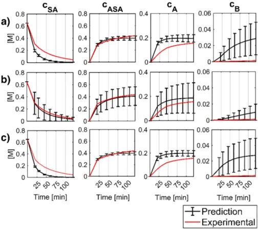
The reaction kinetic parameters (Ai and Ea,i) were estimated using the batch and the continuous experimental data for the acetylation step in different combinations and the flow reactions for the quenching step (see Tables 1 and 2). The calculations were performed using the Covariance Matrix Adaptation Evolution Strategy (CMA-ES), an accel- erated global optimization algorithm that improves the chance of finding the global optimum [32]. The objective functions were formed depending on whether the batch or the continuous experimental data was used for parameter estimation. In the case of the batch data, the normalized mean square errors (nMSE) were calculated between the calculated and measured concentrations for SA, ASA, Impurity A and Impurity B. Normalization of the error components was performed by the difference between the maximum and minimum of the concentration for each component, so that each error component had equal weight in the objective function, irrespective of its concentration range (Eq. (16)).
nMSEX=
1 K
∑K
j=1
(cj,X− cm,j,X
)2
max( cm,X
)− min(cm,X) (16)
where cm,j and cj are the measured and calculated concentrations in the jth sample point, K is to the total number of the sample points and X denotes component SA, ASA, Impurity A and Impurity B. For the continuous experiments, only steady state concentrations were avail- able, from which the nMSEs were further calculated by using normalized concentration values (cnorm,m,j, cnorm,j), where the normalization was done to unit sum (Eq. (17)). This could be reasoned by the fact, that for the simulation of the continuous integrated processes, it is more important to capture the concentrations relative to each other caused by the varying operation parameters, rather than the absolute concentrations.
In this way, information on the absolute concentration is eliminated, but including the nMSEnorm,X terms into the objective function (Eq. (21)) guided the parameter estimation to retain the concentrations relative to the different settings.
nMSEnorm,X=
1 K
∑K
j=1
(cnorm,j,X− cnorm,m,j,X
)2
max( cnorm,m,X
)− min(cnorm,m,X) (17)
where cnorm,j,X= cj,X
∑K
j=1cj,X
(18)
cnorm,m,j,X= cm,j,X
∑K
j=1cm,j,X
(19) Denoting the vector of the considered decision variables by D, the objective functions of the parameter estimation (O) from batch and continuous data took the form:
O(D)batch=nMSESA+nMSEASA+nMSEA+nMSEB (20)
O(D)cont=nMSESA+nMSEASA+nMSEA+nMSEB+w⋅(
nMSEnorm,SA
+nMSEnorm,ASA+nMSEnorm,A+nMSEnorm,B
) (21)
In Eq. (20)-(21), the decision variable D comprises the Ai and Ea,i
parameters of the acetylation and quenching reactions (see Table 6 and 7). In Eq. (21), the weight factor (w) was set to 2 based on preliminary optimizations such as both the absolute concentration values as well as their relative changes through the experiments were satisfactory. When both the batch and continuous data were used for parameter estimation,
the objective function was obtained by summarizing O(D)batch and O(D)cont. The error of fit to the validation experiments was calculated the same way, with the exception that for the continuous samples w=0 were used for a better comparison of the batch and continuous results. In addition to the estimation of nominal parameters, the effects of parameter uncertainties were analyzed on the simulated outputs. This was performed by executing a sufficiently large number of simulations (1000) with kinetic parameter combinations, obtained by Monte-Carlo sampling from the confidence hyper ellipsoid defined by the covari- ance matrix of the nominal parameters [33].
2.2.2. Continuous crystallization
The continuous crystallization of ASA from the reaction mixture was simulated using a one-dimensional population balance model (PBM), developed formerly by the authors of this paper [30]. It was assumed that the kinetics does not depend on the solvent composition. In the previous study [30], various model structures were tested, accounting secondary nucleation, size-independent growth and size-independent agglomeration and it was observed that neglecting agglomeration did not result in considerable performance degradation: the model with agglomeration resulted in 0.770 fitting error as opposed to the 0.772 error obtained without agglomeration, and no visible difference could be observed in the fit of the validation CSDs. For more details see [30].
Since the simulation of agglomeration has the highest computational burden amongst the considered mechanisms, a secondary nucleation and growth PBM was applied. In this way, the PB equation (PBE) took the form of Eq. (22), where the first term on the left-hand side defines Table 5
Constants of the in vitro dissolution model.
Variable Unit Value
mc mg 100
Vd mL 900
ρd kg m−3 1000
td,max min 120
Td ◦C 37
c*d [g ASA/g solution] 3.98 ×10⁻³
Table 6
Estimated kinetic parameters and validation errors for the acetylation with different model structures (95% confidence intervals are in parenthesis).
Model 1 Model 2 Model 3 Model 4
Dataset batch Batch continuous batchþcontinuous
Reaction
schemes Eqs. (1.a, 1.b, 1.c) Eqs. (1.a, 1.c, 1.d) Eqs. (1.a, 1.c (irreversible), 1.d) Eqs. (1.a, 1.c, 1.d)
A1 6.06 £105(3.77 ×10⁴; 9.76 ×10⁶) 4.34 £102(6.46 ×101; 2.91 ×10³) 8.93 £103(1.23 ×10³; 6.46 ×10⁴) 7.48 £102(3.28 ×10²; 1.71 ×10³) Ea,1 56,313(49383; 63244) 38,802(34017; 43587) 48,138(42684; 53592) 40,172(38072; 42273)
A2 1.93 (6.31 ×10⁻²; 5.59 ×101) 0 (fix) 0 (fix) 0 (fix)
Ea,2 28,350(19283; 37417) 0 (fix) 0 (fix) 0 (fix)
A3 3.54 £1016(6.06 ×10¹⁴; 2.07 ×
1017) 2.83 £106(6.79 ×10⁴; 1.18 ×10⁸) 6.28 £106(3.94 ×10⁻²; 9.99 ×
1014) 1.38 £108(3.60 ×10⁻⁹; 5.28 ×1024) Ea,3 124,397(112501; 136294) 62,468(52756; 72180) 74,964(20396; 129533) 70,497(-33965; 174960) Ar3 3.17 £10-14(6.74 ×10³; 1.49 ×10⁻⁵) 4.70 £10-4(2.31 ×10⁻²; 9.58 ×10-
6) 0 (fix) 1.59 £103(8.72 ×10⁻²; 2.89 ×10⁻⁵)
Ea,r3 0 (fix) 0 (fix) 0 (fix) 0 (fix)
A4 0 (fix) 2.23 £104(2.34 ×10³; 2.12 ×10⁵) 2.53 £104(1.72 ×10³; 3.71 ×10⁵) 6.46 £104(5.02 ×10³; 8.32 ×10⁵)
Ea,4 0 (fix) 53,862(48025; 59700) 56,114(49473; 62755) 56,601(49975; 63228)
Errorb 1.36(0.63; 2.29) 0.79(0.41; 1.70) 0.86(0.17; 2.78) 1.02(0.48; 2.15)
Errorc 95.0(73.7; 113.1) 35.4(19.3; 57.6) 46.8(11.8; 97.6) 42.5(23.2; 71.4)
Table 4
Constants and kinetic parameters of the crystallization model.
Variable Unit Value
kv – π/6
ρc kgm−3 1400
Vc m3 2.35 ×10⁻⁴
kb # m-3s−1 3.48 ×10⁶
b – 0.928
kg ms−1 8.51 ×10¹¹
Ea,g Jmol−1 97,323
Table 7
Estimated kinetic parameters and validation errors for the quenching and dissolution models (95% confidence intervals are in parenthesis).
Quenching Dissolution
A5 1.44 £105(1.15 ×10⁵; 1.82
×105) kd 1.98 £10-7(3.14 ×10⁻⁷; 1.25
×10-7) Ea,5 55,595 (fix) d 0 (fix)
A6 0 (fix) p1 1 (fix)
Ea,6 0 (fix) p2 0 (fix)
A7 1.49 £107(9.19 ×10⁶; 2.41
×107) Error 68.73
Ea,7 84,153 (fix)
A,r7 8.22 £101(8.27 ×100; 8.17
×102)
Ea,r7 45,883 (fix)
Error 1.90(1.57; 2.35)
the temporal evolution of the crystal’s population density function (n(L,t), denoting the number of crystals in the L,L+dL crystal size domain at t time) and the second term takes into account the effect of crystal growth. The right-hand side stands for the nucleation and the in- and outflow of the continuous system, respectively.
∂n(L,t)
∂t +G∂n(L,t)
∂L =Bδ(L− Ln) +nin(L,t) τc
− n(L,t)
τc (22)
In Eqs. (22), L denotes the crystal size [m], t is the time [s], G is the rate of crystal growth [m s−1], B is the rate of nucleation [#m−3 s−1], nin(L,t)is the number density function of crystals in the feeding stream [#m−4], τc is the mean residence time in the crystallizer [s], Ln is the nuclei size [m] and δ is the Dirac-delta function. Ln has a very small, practically zero value, therefore it was neglected in the calculations.
The initial condition (Eq. (23)) of the PBE gives the initial CSD n0(L) in the crystallizer, whereas the boundary condition states that the crystals have a finite size (Eq. (24)).
n(L,0) =n0(L) (23)
n(L→∞,t) =0 (24)
The secondary nucleation (Eq. (25)) is expressed as the function of the second moment of the distribution (μ2 [m2 m−3], (Eq.(27)) and the relative supersaturation (σc) [-] (Eq.(27)).
B(σc,μ2) =kbσbcμ2 (25)
μ2=
∫∞
0
L2n(L,t)dL (26)
σc=cc
c*c− 1 (27)
In Eqs. (25)-(27), kb and b denote the nucleation rate coefficient [#
m−3 s−1] and the nucleation rate exponent [-], respectively. c*c is the solubility [kg m−3], which, in the case of a combined cooling-antisolvent crystallization, is dependent on the crystallization temperature (Tc [◦C]) and the antisolvent volume fraction v [-][30]:
c*(Tc,v) =54.51− 118.1v+69.55v2+2.078Tc− 2.459vTc (28) The growth rate is described as a function of the relative supersat- uration and a temperature-dependent rate factor (G0(σ,Tc)), as expressed in Eq. (29), where kg denotes the growth rate coefficient [m s−1], Ea,g represents the activation energy of growth [J mol−1].
G0(σc,Tc) =kgσcexp (− Ea,g
RTc
)
(29) Along with the PBE, the corresponding mass balances were solved for the solute concentration (Eq. (30)) and antisolvent volume fraction (Eq.
(31)).
dcc
dt = − ρckv
( BL3n+3G0
∫Lmax
0
L2n(L,t)dL )
+cin,c− cc
τc (30)
dv dt=vin− v
τc (31)
where ρc [kg m−3] and kv [-] represent the crystal density and volumetric shape factor, respectively. The mass balances have the c(0) = c0 and v(0) =v0 initial conditions, which give the initial solute con- centration and solvent composition in the crystallizer.
A semi-discrete implementation of a high-resolution finite volume method (HR-FVM) was applied to solve the growth part (convective flux) of the PBE [34], simulating the CSD in the range of 0–2000 μm on a uniform grid with 500 cells. The constants used for the simulations are summarized in Table 4. For further details about the crystallization model development, the reader is referred to [30].
2.2.3. In vitro dissolution prediction
The in vitro dissolution of the obtained ASA crystals was described using a population balance model. It could be assumed, that in the USP apparatus the temporal evolution of the n(L,t) population density function (i.e., the number-based CSD) is only affected by the dissolution of the particles. Therefore, the PBE takes the form of
∂n(L,t)
∂t − D∂n(L,t)
∂L =0 (32)
where D is the rate of the dissolution [m s−1] and the same initial and boundary conditions (Eq. (23–24)) apply as for the crystallization PBM.
The calculation of the initial population density [# m−4] from the normalized (measured or simulated) CSD is summarized in the Appendix.
The size-dependent dissolution rate is defined as
D(σd,L) =kdσdd(1+p1L)p2 (33)
where kd and d denote the dissolution rate coefficient [m s−1] and the dissolution rate exponent [-] and p1 and p2 are coefficients indicating the size-dependence of the dissolution. σd is the relative supersaturation, expressed in the same manner as for the crystallization model (Eq. (27)).
Based on literature data [35,36], the solubility of ASA (c*d) in the 0.1 N HCl dissolution medium was approximated as 4 mg mL−1, which was further converted to mass fractions. As the dissolution tests were con- ducted by dissolving 100 mg ASA in the 900 mL dissolution medium (i.
e., the maximum concentration is 0.11 mg mL−1), this means, that experimentally the sink condition criteria met (i.e., dissolution media can dissolve at least 3 times the amount of drug that is the dosage form).
Nevertheless, the supersaturation was accounted in Eq. (33) for the sake of better generalization of the model but is not expected to have a sig- nificant effect in the studied case. As the dissolution tester maintains a constant dissolution temperature (Td) of 37 ◦C, the temperature dependence solubility is neglected.
Along with the PBE, the mass balance for the solute concentration was formulated as Eq. (34), with the initial condition of c(0) =0. dcd
dt =3ρckv
∫∞
0
D(σd,L)L2n(L,t)dL (34)
where cd denotes the ASA concentration in the dissolution medium.
From Eq. (34), the dissolution curve was obtained as DR(t) =cd(t)(mc+ρdVd)
mc
⋅100 (35)
where mc, Vd and ρd correspond to the sample mass [kg], the volume of the dissolution medium [m3] and the density of the dissolution me- dium [kg m−3]. The values of these parameters were chosen based on the experimental method (see Section 2.1.3) and summarized in Table 5. DR
[%] is the dissolved ratio, expressed as the percentage of the total sampled mass. Corresponding to the experiments, the dissolution was modeled for td,max =120 min and during the integrated simulation the time (T85) needed to reach the 85% DR was also calculated.
Similar to the crystallization model, a semi-discrete implementation of a high-resolution finite volume method (HR-FVM) was used for solving the PBE using the same computational grid. The parameter estimation was performed using the calibration powder samples sum- marized in Table 3 and using the root mean square error (RMSE) be- tween the measured and calculated concentration values as an objective function (O(kd,d,p1,p2)d).
O(kd,d,p1,p2)d=
̅̅̅̅̅̅̅̅̅̅̅̅̅̅̅̅̅̅̅̅̅̅̅̅̅̅̅̅̅̅̅̅̅̅̅̅
∑Kd
j=1
(DR,j− DR,m,j
)2
Kd
√√
√√
√ (36)
where DR,m,j and Kd denote the measured dissolved ratio and the total number of the sampled time points, respectively.
For the sake of simplicity in the integrated simulation, it was