Topology and differential geometry

(1)

Topology and differential geometry

Miklós Hoffmann

(2)

Topology and differential geometry

Miklós Hoffmann Publication date 2011

(3)

Chapter 1. Foundations of topology

Topology - in a naive sense - is a field of mathematics dealing with those properties of shapes, which remain invariant under continuous deformations, such as stretching, bending etc. It is important, that no tearing and glueing are allowed. These deformations, mappings evidently alter all of the metric properties - no distances, angles, ratios remain invariant. These transformations radically differ from the well-known geometrical transformations, such as congruence, affinity etc., where some metric invariants are always found.

In this section we follow an easy-to-imagine, less abstract way of describing topology, but there are also properties, which cannot be visualize in our space. Several notions are known from our earlier studies, such as geometry and graph theory - these notions, some of them will be topological invariants - get special view in the context of topology.

1. The topological space

In this subsection we first define the space that we are dealing with. The topological space is a much more generalized notion than geometrical (Euclidean, projective) spaces, since no metric properties are necessary to be defined, only the notions of neighborhood and separation must be described to reach the central notion of continuity.

Definition 1.1.

Let be a non-empty (point)set and let be a family of subsets of . The set together with is called a topological space, if

• The empty set and itself are in

• The intersection of finitely many members of is also in

• The union of any collection (with possibly infinitely many members) of is also in . is called a topology (or a topological structure) on the base set . Elements of are called points here, although theoretically they can be any objects, while members of are called open sets of . If an open set contains a point, then it is called a neighborhood of the point.

The topological space is denoted by .

A set of points will thus be a topological space, if some of its subsets are considered to be open sets. This is a very general notion that can be constrained, if the points of the set are supposed to be separated by disjoint open sets (this assumption looks very natural, although there are spaces which do not fulfill this requirement).

Definition 1.2. The topological space is called a Hausdorff-space if for any two points of the space there are disjoint neighborhoods such that

The well-known spaces such as Euclidean, affine or topological space are all Hausdorff-spaces. From now on, by topological space we mean Hausdorff-space.

2. Topological transformations

As it was mentioned in the introduction of this section, topological transformations are based exclusively on continuity as invariant property. The notion of continuity is known for us from analysis where its definition has been based on distances, but now, we have no metric tools, thus we have to reformulate the definition of continuity.

Definition 1.3. A mapping between two topological spaces is continuous if the inverse image of any neighborhood of the image points (that is any open set containing ) is a neighborhood containing :

(6)

Foundations of topology

Now, we can define the basic map between topological spaces.

Definition 1.4. A map is called a topological map or homeomorphism if it is a 1-1 map, and continuous in both directions. Two subsets of the topological spaces are called topologically equivalent if there exists a homeomorphism which transforms the subsets onto each other.

The homeomorphism is required to be continuous in both directions. Visually it is important to avoid both tearing and glueing during the transformations. If the homeomorphism would be continuous only in the original direction, then tearing would be avoided since around the tearing continuity would be destroyed, but avoiding glueing requires continuity in the opposite direction.

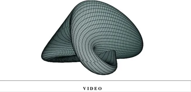
Here we note, that a homeomorphism of a surface cannot necessarily be executed by continuously deforming the surface in the space (See Figure 1.1 and the next video). Those homeomorphisms, which can be done by continuous deforming, are called homotopy.

Figure 1.1. A surface (Boy’s surface) homeomorphic to the projective plane. Although they are homeomorphic, there is no homotopy to transform the projective plane to the Boy’s surface

V I D E O

A homeomorphism is a 1-1 mapping, thus homeomorphism of the space onto itself can be called transformation.

This transformation is - analogously to the well-known ones - is of central importance in topology. Fundamental question in topology is to find invariants under homeomorphisms.

3. Topological transformations

In this subsection properties of curves and surfaces will be discussed that are invariant under a topological transformation (homeomorphism). But first, we have to define what we mean by curve and surface in the topological space, for which we need the (topological) notion of dimension. Dimension has already been studied in linear algebra, where it was the number of elements of a basis in a vector space, but here, in topology, the dimension is defined in a rather different way.

Definition 1.5. Given a topological space . Point elements of this space and any sets of its discrete points are defined as of dimension 0. A subset of the space in one of its points is called of dimension if for any neighborhood of there is a dimensional subset which separates the point and points of out of this neighborhood, but there is at least one neighborhood of where this separation cannot be done by a subset of dimension less than

.

(7)

Foundations of topology

Note that the above definition is a recursive one, that is the dimension is defined by the help of dimension . It is also important that the dimension is assigned to a point of the subset. The whole subset is called of dimension , if it is of dimension in each point.

Definition 1.6. Bounded, closed, connected subsets of a topological space are called curves if they are of dimension 1 in each point, or surfaces if the dimension is 2 in each point. Union of finite numbers of these kind of subsets are also called curve and surface, respectively.

Before studying topological invariants of curves, we remind the reader that we suppose that he/she is familiar with the notions of graph theory. Since two graphs are identical if their vertices and edges can be correspond to each other in a 1-1 way, it is evidently related to the equivalence of topological curves.

Thus the following statements are direct consequences of graph theoretical issues.

Theorem 1.7. The following properties are invariant under a homeomorphism of a curve:

• number of components, that is the number of disjoint parts of the curve

• indeces of points, that is how many branches of the curve pass through a given point

• planarity, that is the fact if there is a curve in the plane which is identical to the original curve

• unicursality, that is the fact if the curve can be drawn by one single line

• number of parts of the plane which are separated by the planar curve

Concerning this latter problem the most famous statement is the Jordan theorem, which states that every planar curve which is homeomorphic to a circle divides the plane into two disjoint parts.

(8)

Chapter 2. Topology of surfaces

In this section the same questions arise in one dimension higher concerning surfaces. Analogously to the curve case, we try to find properties that are invariant under a homeomorphism. Surprisingly one of the most important topological invariants, the Euler characteristic, has originally been studied in elementary geometry, in the field of polyhedra, as an expression of the sum of the edges, vertices and sides.

1. The Euler characteristic

Before starting to study surfaces, we will restrict the notion of surface. Originally, a surface is a two dimensional topological object, but we will focus on those surfaces that are homeomorphic to a disk, or can be constructed by glueing together such surfaces. By glueing we precisely mean that a part of the boundary of a disk is joined to a piece of boundary of another disk, or to another part of the boundary of the same object such that at every joint two and only two disks are joined. If the surface is bounded and all of its points are interior point, then the surface is called a closed surface.

Based on the previous restrictions, one can draw a graph onto the surface in a way that the surface is divided into pieces homeomorphic to a disk. For simple polyhedra this graph can be the graph containing the vertices and edges of the polyhedra itself. It has been proved (c.f. Euler theorem for polyhedra) that if the number of vertices, edges and faces (disks) are denoted by and , respectively, then .

This theorem is a special case of a more general statement. The graph can be drawn onto any surface and the number of vertices, edges and faces (pieces homeomorphic to a disk) will be formulated in a similar way.

Theorem 2.1. Consider the graph drawn onto the surface. Let the number of vertices, edges and faces (pieces cut by the edges, homeomorphic to a disk) be , , and , respectively.

Then the number is independent of the graph itself, depends only on the surface.

Definition 2.2. The number is called the Euler characteristic of the surface .

The Euler characteristic typifies the surface, but a much stronger statement also holds: it is a topological invariant.

Theorem 2.3. If two surfaces are topologically equivalent (homeomorphic), then their Euler characteristics are identical.

Let us see some examples. The Euler characteristic of the sphere, as it directly follows from the original Euler theorem for polyhedra, is . For the disk itself , since choosing a point on the circle as vertex, the circle itself will be the only edge, while the disk is the only face, thus .

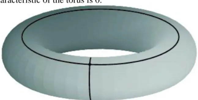
Figure 2.1. Euler characteristic of the torus is 0.

The Euler characteristic of the torus can also be computed by drawing a simple (as simple as possible) graph. As

it can be seen in Fig. 2.1, .

As a last example, let us consider the Möbius strip (see Figure 2.2 and the next video).

Figure 2.2. Euler characteristic of the Möbius strip is 0

(9)

Topology of surfaces

V I D E O

The boundary of the strip is homeomorphic to the circle, thus choosing a point on it the number of both vertices and edges would both be one. But the generated graph is not suitable, since the face is not homeomorphic to the disk - for this we need a further edge (like cutting the strip) and another vertex, having two vertices, three edges and one single face (like a quadrangle), conversely the Euler characteristic is .

These latter two examples warn us that Theorem 2.3 does not hold vice versa: the fact that two surfaces have the same Euler characteristic, does not implies that they are homeomorphic, since e.g. the torus and the Möbius strip are evidently not topologically equivalent (the strip is of one-sided, while the torus has two sides).

For a more complicated surface one may have to draw a complicated graph as well. But the Euler characteristic can be computed by dividing the surface into simpler parts and adding the individual characteristic in a certain way. The following theorems help us to do so.

Theorem 2.4. If we cut a disk out of a surface, then the Euler characteristic of the new surface is one less than the Euler characteristic of the original surface.

Proof. Consider a graph on the surface such that the disk in question is a face of this graph.

After cutting the disk out, the number of edges and vertices remain unchanged, while the number of faces will be one less. Thus the sum will also be one less and this was to be proved. □

Theorem 2.5. Consider two surfaces and with boundary, the boundaries are homeomorphic to the circle. Let . Then glueing them along their boundaries, the new unified surface has Euler characteristic: .

Proof. The statement can also be formulated in a way that we glue the hole (homeomorphic to a disk) in by the other surface . We can draw a graph onto both surfaces in a way that the boundaries contain one vertex and thus one edge. At glueing we can assign the vertices in the two boundaries and the two boundaries themselves to each other. Thus the union of the two graphs will be a suitable graph in the surface to compute the new Euler characteristic.

But at the glueing process only one vertex and one edge disappeared, all the others remained

unchanged, hence . □

Theorem 2.4 is obviously a special case of Theorem 2.5. The two statements together give us a possibility to glue closed surfaces and compute the Euler characteristic of the new surface. Consider two closed surfaces and with Euler characteristics . Cut a region homeomorphic to a circle out of both surfaces, and glue them along the boundary. Due to the previous computations, cutting makes the Euler characteristics of both surfaces one less, while glueing yields a simple addition. Thus the Euler characteristic of the final surface is .

Example 2.6. Consider a sphere and a torus. Cutting a circle out of both surfaces and glueing them along the boundary, the new surface - sphere with handle - has Euler characteristic . The same computation can be done by cutting out circles and glueing them

(10)

by tori. The resulted surface is called sphere with handles, and its Euler characteristic

is .

Example 2.7. Consider again a sphere and cut out disjoint disks. Now, the holes are closed by no tori but by Möbius strips. As we have mentioned, the boundary of the Möbius strip is homeomorphic to the circle, that is it is possible to close the hole with it, although there is no homotopy which transforms the Möbius strip to a surface with planar circle boundary. These surfaces are denoted by and their Euler characteristics are . Note that these are one-sided surfaces.

Figure 2.3. The Möbius strip can be topologically transformed to a surface with circle boundary, although it is not a homotopy

Although a homeomorphism, which is not a homotopy, is very hard to visualize, Figure 2.3 tries to explain the transformation of the Möbius strip to a surface with circle boundary.

During this construction we cut and glue, which is not allowed in a homeomorphism, but at the final stage the boundaries of the separated parts coincide again from point to point, thus the first and the final shapes are homeomorphic.

Here we note, that the projective plane can be constructed in a similar way. The projective plane can be considered as the extension of the affine plane by ideal elements. In this extension the topology of the plane will be changed rather drastically by glueing the lines in their ideal point to a circular shape. If we imagine the affine plane as a disk with boundary, then glueing the opposite points of this boundary we can obtain the projective plane. This can be done by deforming the disk to a hemisphere, and then close it by a surface homeomorphic to Möbius strip and having circular boundary, just as the surface we have constructed before. Thus the projective

(11)

plane is homeomorphic to a sphere with one hole closed by the Möbius strip, which has been denoted by . It is interesting to note, that the projective plane, such as , is a one-sided surface. In the three dimensional affine space we cannot provide a surface homeomorphic to the projective plane without self-intersection, but in Figure 1.1 one can observe the complexity of this surface - this is a famous surface homeomorphic to the projective plane.

One may think that beyond these examples many-many more surfaces can be constructed by glueing and cutting. This is why the following theorem, proved by Möbius and Jordan sounds surprising and us of central importance providing the topological classification of closed surfaces.

Theorem 2.8. Any closed surface is homeomorphic to one of the following surfaces:

, where is a sphere with holes and closed by tori, while is a sphere with holes closed by Möbius strips.

Proof.

We did not completely prove the theorem, only give some remarks. It is easy to prove, that all the surfaces mentioned in the theorem are different from a topological point of view. Surfaces have different Euler characteristics depending on , surfaces also have different characteristics depending on . Two surfaces and can have the same Euler characteristic, but is a one-sided surface, is a two-sided surface, and this property is a topological invariant. If we would try to construct a new surface by cutting holes and closing of them by tori, while of them by Möbius strips (where ), then it will be equivalent to a sphere with holes closed by Möbius strips, that is homeomorphic to the

surface .

The deep part of the proof is to show that any closed surface is homeomorphic to one of the above mentioned surfaces, but this is not proved here. □

2. Topological manifolds

After curves and surfaces we will study a more abstract and general notion, namely the manifold. Manifolds are locally homeomorphic to the dimensional Euclidean space, more precisely every point has a neighborhood, which is homeomorphic to an open set of . This means, that manifolds can "piecewisely" be considered as Euclidean space, but they can be very complicated structures. In this subsection we shortly mention some important notions and results about manifolds.

Definition 2.9. A topological space or a subset of it is called dimensional topological manifold (or simply manifold), if every point has a neighborhood, which is homeomorphic to an open subset of .

To understand the locality of the definition, consider a simple example. The circle is a one-dimensional manifold, because, although it is not homeomorphic to any open set of (that is not homeomorphic to any open interval of the line), but each point of the circle evidently has a neighborhood, for example a semicircle, which is homeomorphic to an open interval.

Analogously, the sphere or the torus is a two-dimensional manifold, because every point has a neighborhood (for example a small circular part on the surface), which is homeomorphic to the open disk.

A three dimensional manifold is, for example, the three dimensional sphere or simply 3-sphere, which contains all of the points of the 4 dimensional Euclidean space which are of a fixed distance from a given point.

It is easy to prove that every simply connected, closed one dimensional manifold is homeomorphic to the circle, and every simply connected, closed two dimensional manifold is homeomorphic to the sphere. The analogous statement is a very hard problem in higher dimensional spaces, which has been proved recently for dim .

Theorem 2.10 (Poincaré - Perelman). Every simply connected, closed three dimensional manifold is homeomorphic to the 3-sphere.

This statement was known as Poincaré-conjecture until 2003, when Perelman proved the theorem. It is interesting, that for dimensions higher than 3 the proof is much easier.

(12)

3. The fundamental group

In this subsection we study paths in a topological space or along a manifold. By path we mean the trace of a point which runs from a given point to another given one continuously in the space or in the manifold. Based on this study we can define an algebraic group which is assigned to the space and is of great importance.

Definition 2.11. Consider a topological space and one of its points . The paths starting and ending at are continuous mappings for which . Two paths are equivalent if there is a homotopy between them in the given space.

If the point of the space is fixed, then the homotopy of paths starting and ending at the given point are called loops. The homotopy of loops generates an equivalence relation, since it is reflexive (any path is homotopic to itself), symmetric (if path is homotopic to path , then, due to the 1-1 mapping, it holds vice versa)and transitive (since homotopy is transitive). Thus this relation induces a classification in the set of loops having equivalent loops in one class. Among these classes one can define an operation by running along the two loops one after another. This operation is called concatenation. Let this operation be denoted by , which means that we runs along the loop from the given point and when we arrived back at , we start to move along the loop arriving back again to , and this is again a loop.

Theorem 2.12. Homotopy classes of a topological space generated by the point form an algebraic group for concatenation as operation.

Proof. As we have seen, the set of classes is closed for the concatenation. Consider the class containing those loops which can be contracted to one single point. This class is the identity element. Every loop has its inverse, running along the same loop backwards, which is again a loop, and concatenating it to the original one, we obviously obtain a loop from the identity element. It is also easy to see that associativity holds, since passing through again and again it is irrelevant which loop we will follow next. □

It is important to note, that the above group is not commutative in general. Another question arises: if we consider another starting point of the space, having other loops, whether this group will be similar to the previous one?

Theorem 2.13. Any two points and of a topological space generate isomorphic groups.

Proof. Consider a path connecting and , let us denote it by . For every loop starting from assign the loop starting from , for which , where is the same as but backwards. This map is a 1-1 map between the (classes of) loops, moreover it is

an isomorphism: for any two loops and

. Hence the two groups are isomorphic. □

After this theorem the group can be assigned not only a specified point of the space, but the space itself.

Definition 2.14. The group generated by the loops of a point of the topological space is called a fundamental group of the space.

Fundamental groups are important tools because they can describe the structure of the space, as one can observe from the following theorem.

Theorem 2.15. Two topological spaces are homeomorphic their fundamental groups are isomorphic.

This allows us to study the topology of manifolds and spaces by the algebraic structure of their fundamental groups, which is, as we have seen, topological invariant. Thus the fundamental group of the disk and the sphere contains only one element, the identity element, because for any point all the loops can be contracted to that single point.

Figure 2.4. Loops on the disk can be contracted to one single point - the fundamental group contains only one element, the identity element

(13)

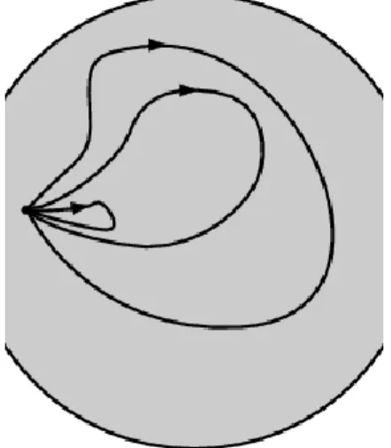
However, if we cut a hole into the disk, or omit a single point of the sphere, the fundamental group will suddenly have infinitely many elements. One class contains those loops which go around the hole or the missing point times, where . Thus this fundamental group is isomorphic to the additive group of integers.

Figure 2.5. Loops of the disk with a hole cannot be contracted to one point. Loops going around the hole times form one class, for we have the identity element. This group is isomorphic to

Finally the fundamental group of the projective plane has two elements, loops are in one or in the other class depending on whether they intersect the line at infinity or not.

(14)

Chapter 3. Foundations of differential geometry, description of curves

A broad class of curves and surfaces will be studied in this section, mainly by analytical tools. This approach makes us enable to describe those properties of curves and surfaces, that can be examined hard by algebraic tools. Due to the basic properties of differentiation, however, our results will hold only in a sufficiently small neighborhood of a point, that is our results will almost exclusively be local results.

First we have to define what type of curves will be studied here, more precisely we have to describe what we mean by curves in terms of differential geometry.

We can think of a space curve as a spatial path of a moving point. At any moment of the movement draw the vector from origin to point . Let us denote this vector by . This way we have a vector-valued function, defined on a (finite or infinite) interval (c.f. Fig. 3.1). This vector-valued function is, in general, not a 1-1 mapping, there may be parameters for which , . This is a double point of the curve, where the curve intersects itself. To eliminate these points in the future, we assume that the function is a 1-1 mapping. It is also desired to consider only continuous functions, more precisely functions which are continuous in both directions. This means that if a sequence in the interval converges to , then the point sequence is also convergent and converges to and vice versa. A 1-1 mapping, which is continuous in both directions, has been called topological mapping.

Figure 3.1. Definition of a curve as a scalar-vector function

Definition 3.1. By curve we mean an scalar-vector function defined on a finite of infinite interval that satisfies the following conditions a) is a topological mapping b) is continuously differentiable on c) the derivative of does not vanish over the whole domain of definition.

The scalar-vector function is a representation of the curve, but this curve can also be described by other functions as well, some of them may not fulfill all the conditions mentioned above. Those representations that fulfill conditions a) - c) are called regular representations.

Function will normally be given by its coordinate functions . Derivative of is also computed by differentiating the coordinate functions. The derivative function, which itself is a scalar-vector function as well, is denoted by .

Concerning the definition of curves we have to emphasize that the word "curve" is frequently used in everyday life and it very often indicates shapes that do not fulfill the requirements we gave. These requirements are especially defined because we want to apply analytical tools above all differentiation.

Example 3.2. The function is an equation of a straight line, where is a point of the line, while is a direction vector of the line. By coordinate functions:

Example 3.3. Function defines a circle, where is the

center of the curve, the plane of the circle is given by the orthonormal basis with origin and

(15)

Foundations of differential geometry, description of curves

unit vectors , while denotes the radius of the curve. For the parameter

. Specifically the circle with origin as center, , as unit vectors and as radius is given by the following coordinate functions:

Example 3.4. The function defines a helix in the orthonormal basis, where is a constant, which is the height of one complete

helix turn, called pitch. Using coordinates , , the

coordinate functions of the helix are:

The function uniquely determines the curve, but not vice versa: a certain curve has many - and many regular - representations, there are infinitely many functions that define the same curve. Consider a real function between two given intervals. If , then is the very same curve, as . This way we transform the representation to by the help of . This technique is called a parameter transformation.

Example 3.5. In example 2) we defined a circle on the interval . Now we transform the parameter to applying the transform function . Hence

Theorem 3.6. A parameter transformation transforms a regular representation to a regular representation again, if and

If a parameter transformation works on a curve as it is written in the theorem, then it is called an admissible parameter transformation. If we consider a direction on the curve determined by increasing values of the parameter, then it is called an orientation of the curve. Two representations, and of the same curve determine the same orientation, iff the transformation function which transforms to the representation is a strictly increasing function. If is strictly decreasing, then the two representations have opposite orientations.

If all the points of the curve are in one single plane, then it is called a plane curve, otherwise it is a spatial curve.

1. Various curve representations

In the preceding section we have seen the parametric representation of curves. However, there are other methods to describe a curve. In school two elementary methods are preferred, the implicit and explicit way of definition.

For plane curves these representations are as follows:

1.

Explicit representation.Consider a Cartesian coordinate-system in and the function . Those points, the coordinates of which fulfill the equation, form a curve. This representation is called Euler-Monge-type representationof the curve.

2.

Implicit representation.Consider a Cartesian coordinate-system in and the function . Those points, the coordinates of which fulfill the equation , form a curve. Note, that the points fulfilling

(16)

the equation (where ) also form a curve. This representation of the curve is introduced by Cauchy.

3.

Parametric representation.This is the method of curve representation what we described in the definition. The curve is given by the parametric form which has two (or in space three) coordinate functions:

This form is frequently referred to as Gauss-type representation.

Each of the forms above have their advantages and drawbacks. The explicit form cannot be considered as universal description, e.g. the equation of a straight line cannot represent the lines parallel to the axis. The first two forms cannot directly be applied for spatial curves, hence introducing a new unknown, and represent surfaces instead of spatial curves. In this sense the parametric form is the most general representation form of the curves.

Conversions between different forms yield problems of very different level of difficulty. While transfer the curve from explicit representation to implicit form simply means a rearrangement, the transfer from implicit form to explicit representation requires deeper mathematical background. The theoretical possibilities of conversion will be discussed in detail when examining the surfaces, now, we show only an example for polynomial curves.

2. Conversion between implicit and parametric forms

Now, we consider only polynomial curves. The two opposite directions of this conversion have different mathematical difficulties. From parametric form to implicit form the conversion is always possible theoretically, however there can be practical problems at the computation. A planar curve or a surface given by implicit equation does not necessary have parametric representation though, and even if it exists, there is no universal effective method to compute it. For spatial curves, which are given in implicit form by the intersection of two implicitly given surfaces, the parametric form does not necessarily exist even in the case when the two surfaces have this kind of representations.

The simpler case is to convert the parametric form to implicit one. It is based on the fact that the coordinate- functions of the parametric form can be considered as a system of equations, in which the unknowns are for planar curves, for surfaces. If we eliminate the unknown (or unknowns for surfaces), then the equation we obtain is nothing else then the implicit form of the object. The elimination always works theoretically, but for higher degree polynomials computations can be very complicated, thus for practical usage there are faster algorithms for low degree polynomials. We present such a method for planar curves here.

Let a planar curve with coordinate functions be given. In general these functions are rational polynomial functions thus we can write them in the form

where coefficients are real values. Now the implicit form of this curve can be computed by a determinant

where elements of the matrix are

(17)

The above determinant is called Bézout–resultant and it provides a simple algorithm for planar curves. Note that the degree of the equation (i.e. the order of the curve) has not been changed by the conversion.

Similar algorithm exists for surfaces, but for spatial curves, where the implicit and parametric forms are essentially different, this method does not work.

Conversion in the opposite direction, as it is mentioned, yields a more difficult mathematical problem. There is no general, universal method even for its existence, that is for deciding whether there is at all a parametric form of an algebraic curve given in implicit form. The most known result about it is a theorem by Noether, in which the genus of the curve plays an essential role:

where is the order of the algebraic curve, while is the number depending on the number of singular points of the curve (here the curve is considered above ).

Theorem 3.7. (Noether) An algebraic planar curve given in the form has parametric form iff genus

This theorem solves the problem of existence theoretically, but the computation of genus is not always a trivial task, and even if it is computed, the theorem does not provide a constructive way to find the parametric form. Similar theorem exists for surfaces (Castelnuovo-theorem), but neither of these theorems gives us a constructive approach. For certain types of simple curves, which are important in everyday practical applications, for example for conics and for some cubic curves, there are practical algorithms to compute the conversation. One of these algorithms is discussed in the next section.

3. Conversion of conics and quadrics

For any non-degenerated conics there exists a parametric form. The method, converting the implicit form to parametric one, is based on the fact that if a line intersects a conic in a point, then there must be another intersection point as well. In Euclidean plane there are two exceptions: the parabola, where lines parallel to the axis of the parabola intersect the curve only in one single point, and the hyperbola where lines parallel to the asimptotes intersect the curve in a single point as well. These exceptions, however vanish in the projective plane, where these lines intersect these curves in two points, one of which is at infinity.

Let us choose an arbitrary point at the conic and consider the family of lines passing through this point. Each element of this family intersects the conic in a point different from . If we describe the family by the help of a parameter , then this parameter can also be associated to the intersection points, i.e. to the curve points except . Let the parameter being associated to . This way we obtain the complete parametrization of the curve.

Follow this idea in the case of a simple example, so consider a circle with unit radius and with center at the origin. The implicit form of this curve is

Let us choose the point of this curve. Lines in the form passing through are of the form . Thus the equation of the family of lines passing through is

(see Fig. 3.2).

Figure 3.2. A possible parametrization of the circle

(18)

These lines intersect the circle in and in another point, say . This point evidently depends on the parameter . One can easily compute the coordinates of the intersection point if we substitute the equation of the line to the equation of the circle:

from which

where root provides the original point , while the other root (more precisely the coordinate obtained by the backward substitution) provides the other point . The coordinates of this point (depending on ) are:

Because of altering the straight line, point runs on the circle, the system of equation described above provides the parametric representation of the circle.

The parametric equation of any non-degenerated conics can also be computed by an analogous technique. The following table shows the parametric equations of these curves.

All of the non-degenerated conics of the plane can be transformed to one of the above mentioned form (so- called canonical form) of curves by coordinate-transformations. Thus a curve can also be parameterized by

(19)

transforming it to canonical form, and then applying the inverse of this transformation to the above parametric equation.

Concerning parametrization problems, the described method is not unique, for example, in technical studies there are other types of parametrization techniques for special curves.

Finally, we remark that the method described above can also be applied for those algebraic curves of order , which have an -tuple point (also called monoids). Lines passing through this point intersect the given curve in one single point as well, thus the parametrization can be computed (see for example the cubic curve with double point in Fig. 3.3).

Figure 3.3. This cubic curve with double point can be parametrized by the described method:

.

The problem of finding the intersecting points of two planar curves can ideally be solved in the case when one of the curves is given in implicit form, while the other curve is given in parametric form. Other cases can be computed by transferring the problem to this case by parametrization or implicitization.

Consider two planar curves, one of them is given in implicit, the other one is given in parametric form:

Substituting the coordinate equations of to the implicit form of the following equation holds:

the degree of which is the product of the order of the two given curves. Roots of the equation falling into the domain of definition of give us the parameter values associated to the intersection points of the two curves.

Substituting these values to the equations of the coordinates of the intersection points are obtained.

(20)

Chapter 4. Description of parametric curves

1. Continuity from an analytical point of view

Let us consider two curves, and , meeting at a point . Due to the traditional concept of continuity the joint of two curves are said to be n-times continuous, or in other notation - continuous, if the derivatives of two curves coincide at the given point up to order, that is

are fulfilled.

By the help of this concept one can easily define the continuous joint of a surface and a curve, or two surfaces.

The joint of two surfaces is continuous, if all of their partial derivatives coincide at the intersection points up to order. The joint of a surface and a curve is continuous, if there exists a curve on the surface that is met by the given curve in an -times continuous way.

The continuity of the joint of two curves or two surfaces thus can be checked by simple computation of the derivatives. The continuity of a curve and a surface, however, requires a suitable curve on the surface, which cannot be found in a straightforward way. The following theorem can help us in solving this problem.

Theorem 4.1. Let a surface be given, the derivatives of which exist and do not vanish up to order in any variables. Then the curve , , touches the surface at one of their points times continuously iff there exists a parameter value for which the derivatives of the function fulfill the equation

Proof. Suppose, that there exists a curve on the surface, which touches the original curve in an times continuous way.Then

and the derivatives of the two curves also coincide, from which, applying the fact that

follows, that

For higher derivatives the statement can be proved in an analogous way.

Now suppose, that

holds. Then we have to find a suitable curve on the surface. All the partial derivatives of the surface exist and do not vanish, thus the surface can be converted to the explicit form, say . Projecting the curve onto the surface by a direction parallel to the axis, the coordinate functions of the projected curve are

(21)

Description of parametric curves

and one can easily see that this curve and the original curve meet in a times continuous way.

□

2. Geometric continuity

From a geometric point of view the continuity of two curves means that at the joint point the tangent vectors of the two curves are identical. A less severe condition would be the coincidence of the directions of the two tangent vectors, that is the coincidence of the tangent lines, fulfilling the equation

This latter criteria has a certain advantage over continuity: it is independent of the current parametrization of the two curves, and this condition is formed from a purely geometric viewpoint. This is why this latter continuity is frequently referred to as first order geometric continuity, or continuity.

In a similar manner higher order geometric continuity can be introduced as well. Remember that analytical continuity and continuity require the coincidence of second and third derivatives, respectively. The second and the third order derivatives are applied to describe the curvature and the torsion, respectively, so it is a good strategy to require their coincidence to define the higher order geometric continuity..

Thus two curves at their joint point are said to be continuous, or second order geometric continuous, if the direction of the tangent vectors as well as the curvature at coincide. By applying the definition of the curvature and the criteria of continuity, this requirement can be defined by the following system of equations:

Analogously, two curves at their joint point are said to be continuous, or third order geometric continuous, if the direction of the tangent vectors as well as the curvature and the torsion at coincide. Adding the definition of the torsion to the previous conditions, the criteria of third order continuity can de defined as:

Geometric continuity can be generalized for higher order as well, but only in higher dimensional spaces, where there are further invariants similar to the curvature and the torsion.

Geometric continuity is less restrictive than analytical continuity, but it is defined by purely geometric conditions, independently of the actual parametrization of the curves. It is important to note, that visually the two different notions of continuity cannot be distinguished for order higher than 2.

3. The tangent

Consider a curve and let us fix one of its points , associated to the parameter value . Let

be a sequence of parameter values in the domain of definition, which converges to . This sequence of real numbers defines a point sequence on the curve as well.

Definition 4.2. The tangent line (or simply tangent) of the curve at is defined as the limit position of the lines of the chords if this limit is independent of the choice of the sequence converging to .

Theorem 4.3. At each parameter value of the curve the tangent line uniquely exists.

It is the line passing through the point and having the direction , which is called tangent vector.

(22)

Proof. Consider the lines . These lines form a convergent sequence of lines, because the point sequence tends to the limit point and the direction vectors of the lines also form a convergent sequence. The direction vector of the line is or this vector multiplied by a nonzero scalar. Thus, for example vector is a direction vector. Due to the definition of differentiation, the sequence of these vectors tends to the vector for any sequence of parameters . □

Figure 4.1. Definition of tangent

Based on this theorem, the parametric equation of the tangent line of the curve at the point is:

Example 4.4. Consider the circle with origin as center. Its parametric representation is , . The tangent vectors at the points of the curve

are: . If , then the tangent vector is a vector with

coordinates . The length of the tangent vectors can be determined as:

that is at each point of the circle the tangent vector is of equal length. This length, however, depends on the actual parametrization of the curve - other parametrizations may yield non- constant tangent lengths.

4. The arc length

Consider the curve and its arc which is the image of the segment of the parameter domain I. Let be a partition of the interval. Points of the curve associated to the values of this partition, are . Connecting these points in this order we obtain a broken line inscribed to the curve, which is called normal broken line.

Definition 4.5. Consider an arc of a curve and all the possible normal inscribed broken lines to this arc. The arc length of this arc is the least upper bound (supremum) of the set of lengths of the broken lines mentioned above.

Theorem 4.6. If we consider the arc of the curve from the point assigned to the parameter value to the point assigned to then the length of this arc is

The integrand of the integral in the previous theorem is nothing else than Thus

As we observed, there are infinitely many representations of a curve with various parametrizations. But the statements about a curve should be about the curve itself and not about one of its representations ( i.e. one of its specific parametrizations). We intend to apply a parametrization, which is uniquely determined by the curve,

(23)

thus it has itself some geometric meaning. Arc length is a parameter of that kind. In arc length parametrization, a parameter assigned to a curve point is the measure of the arc length computed from a fixed point to . The measure is signed measure, having a predefined orientation along the curve. It can be proved, that starting from any regular parametrization there is a transformation which yields an arc length parametrization of the curve. One can consider the computation of the arc length of the curve as an integral where the upper end is a variable. Thus the arc length is the function of , the original parameter:

Function is strictly increasing, because it is the integral of a positive function. It is also continuously differentiable, because the integrand is continuous. Thus there exists the inverse function of

which is also strictly monotonous and continuously differentiable. Hence is an admissible parameter transformation of the given curve. Arc length is determined up to an additive constant, which is a consequence of the arbitrary choice of the starting point and its parameter . Arc length parametrization also yields constant tangent vector with unit length.

Various parametrizations of a curve can be considered as various movements along a fixed trajectory. If the parameter is the arc length, then this movement is of unit speed, that is the displacement is proportional to the time. To distinguish arc length parametrization from other regular parametrizations, derivative of the curve is denoted by .

Example 4.7. Consider the helix and compute

its representation by arc length parametrization. The derivatives are , hence the arc length can be expressed as:

which yields . Substituting this formula to the original equation we get

which is the representation of the helix with arc length parametrization.The tangent vector is as follows

The length of the tangent vector can be written as

5. The osculating plane

Consider the curve parametrized by arc length. Let this curve be two times continuously differentiable.

Further on let be an arbitrary point on the curve where does not vanish. Consider three points on the curve, which are not collinear: with assigned parameter values , and let the points

(24)

tend to the point along the curve. At each moment these three points uniquely determine a plane (except at particular cases when these points are collinear for a moment).

Theorem 4.8. Given a curve and three points on it, the sequence of the planes defined by these points as tend to the point , has a unique limit plane, which depends only on the curve and the point . This plane is defined by the vectors

and in .

Definition 4.9. The limit plane defined above is called osculating plane of the curve at .

The equation of the osculating plane can be written by a scalar triple product (which is denoted by parentheses):

where is a vector to a point of the osculating plane. Its components are:

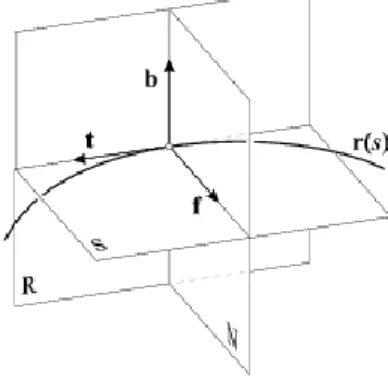
6. The Frenet frame

Figure 4.2. The Frenet frame and the planes determined by the frame’s vectors: the osculating plane (S), the rectifying plane (R) and the normal plane(N)

At each point of the curve a system of three, pairwise orthonormal vectors can be defined. If we consider these vectors as unit vectors of a Cartesian coordinate-system, the description of the curve becomes much simpler. Let the curve be two times continuously differentiable with arc-length parametrization, and suppose that the vector do not vanish at any point. Let the first vector of the Frenet frame be the tangent vector , which is of unit length, due to the arc-length parametrization. Let us denote this vector by . The second vector of the frame will be one of the normals of the tangent vector lying in the osculating plane. The vector is in the osculating plane and derivating the equation we have which means that it is orthogonal to the tangent vector as well. Thus the second vector of the frame can be the unit vector with the direction of , which will be called normal vector, denoted by . The third vector of the frame has to be orthogonal to the first two vectors and , thus it can be the vector product of these vectors. It is called binormal vector. Finally the vectors

form a local coordinate-system at each point of the curve. The coordinate plane of and is the osculating plane, while the plane defined by and is called normal plane, while the third plane, defined by and is the rectifying plane. If holds at a point of a curve, then the Frenet frame cannot

(25)

be uniquely determined at this point. If this is the case along an interval of the parameter domain, then the curve is a line segment in this interval.

(26)

Chapter 5. Curvature and torsion of a curve

Two fundamental notions about the parametric curves will be defined and studies in this section. Curvature provides a value to measure the deviation of the curve from a line at a certain point. Torsion provides a value to measure the deviation of the spatial curve from a plane at a certain point. Curvature and torsion are two functions along the curve, by which - as we will see - the curve is completely determined.

1. The curvature

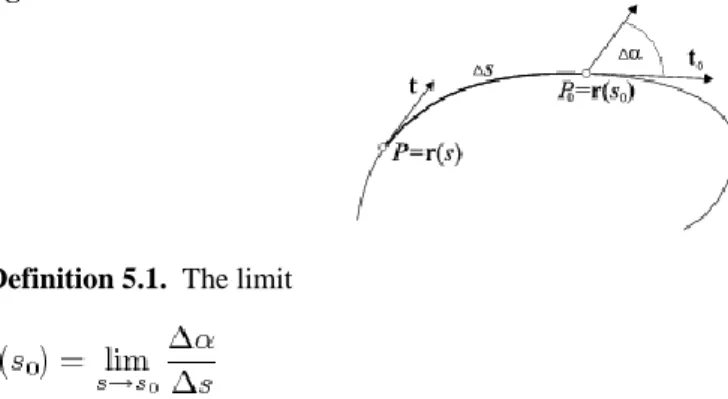
Now curves are planned to be characterized to show how much they are curved, that is by the measure of their deviation from the straight line (which is not curved at all). Tangent lines of the straight line are parallel to (actually coincide with) the line itself and therefor to each other as well. Thus the measure of the deviation can be based on the change of the direction of the tangents. Let be a two times continuously differentiable curve given by arc-length parametrization. Let the tangent vector at point and be and

, respectively. The following notations are introduced: and (see Fig. 5.1).

Figure 5.1. Notion of curvature

Definition 5.1. The limit

is called the curvature of the curve at .

Theorem 5.2. The above defined limit always exists and it can be written as:

Proof. It is known, that the ratio of the angle and its sine tends to 1 as the angle decreases, that is , which yields the following expression of the limit . But the sine of the angle can be written by the help of the

vector product of the unit tangent vectors, because . Thus

Applying the identity of vector products and using the fact that the vector product of any vector by itself is the zero vector, we obtain

(27)

Curvature and torsion of a curve

To prove the formula for curves given by general regular (non-arc-length) parametrization, suppose, that the curve can be transformed to arc-length parametrization by the transformation function . Now is parametrized by arc-length. By the rules of differentiation one can obtain

moreover

Applying the fact, that vectors and are orthogonal and , one can write

Derivative of the transformation function is as

thus finally

from which one can obtain the final formula by substitution

□

Now we describe an important relation between , and . By definition , thus or by other formulation . This latter formula is one of the Frenet-Serret formulas, which will be proved in the following sections.

It is obvious from the definition, that the curvature of any straight line is identically zero, and vice versa: if the curvature of a curve is identically zero, then it must be a straight line. It is easy to show, that the curvature of a circle with radius equals , and it can be shown that every planar curve with non-vanishing, constant curvature must be a circle. As one may expect, the larger the radius of the circle the smaller the curvature of the curve. Finally it is noted, that one can define signed curvature as well, if the angle in the definition of the curvature is considered to be signed.

One can measure the curvature along the whole curve, that is to integrate the curvature function along the curve .

Definition 5.3. The total curvature of taken with respect to arc-length is defined as .

The total curvature has an interesting relation to the topology of the curve. To explore it the Gaussian-map of the curve is needed to study first. Consider the tangent vectors of the curve and their representatives starting from the origin. Assign the endpoints of these representatives to the points of the curve.

Since the curve is parametrized by arc-length, the tangent vectors are of unit length, thus the mapping assigns points of the unit sphere with origin as center to the curve points. The mapping is continuous, the image is uniquely defined, but not 1-1, because the tangent vectors can be parallel at several points of the curve, which are thus mapped onto the same points of the sphere.

(28)

For closed planar curves the image of the Gaussian-map is the whole circle with origin as center. The mapping may cover the circle several times. The number which shows how many times the vector turned around the circle in the mapping, is called rotation index of the curve. The rotation index is denoted by .

Theorem 5.4. The total curvature of a closed planar curve equals the product of and a constant which is actually the rotation index of the curve, that is

Proof. Let the domain of definition of the curve be [0,a], where . Further let be the angle of the axis and the representative of the tangent vector starting from the origin at the Gaussian map. Thus

that is the coordinate-functions of are . Using the rules of

differentiation we obtain , which yields

Compare it to the Frenet-Serret formula, which states, that , one can see, that is nothing else than the curvature function of the curve, from which, by integration, the following integral function as upper end is received

Since our curve is closed, that is the two parametric endpoints coincide, at the endpoint the function takes a product of and a constant which cannot be else than the rotation index, that is

and this was to be proved. □

The Gaussian map is also suitable for studying the behavior of the points of the curve. Algebraic curves and surfaces generally look similar at every point, but in some cases, the curve suddenly changes at a point in some sense. Ordinary points are also called regular points, while extraordinary points are called singular points. Such singular points can be e.g. cusps, isolated points, double points or multiple points. Detecting singular points along the curve is not an easy task, in many cases they can be found by approximating numerical methods. For planar curves the Gaussian map and the behavior of the tangent along the curve can help us in finding singularities.

If the tangent of the curve and the associated Gaussian image are changing in one common direction continuously around a point, then we are in a regular point. If the tangent image has a turn, then we are in an inflexion point. If the tangent direction itself has a turn, then we have a cusp on the curve, more precisely it is a cusp of first type, if the Gaussian map has no turn, and of second type, if the Gaussian image has a turn as well.

One can see some examples in Fig. 5.2.

Figure 5.2. Various types of curve points, from left to right: regular point; inflexion point;

cups of first type; cusp of second type

(29)

Similarly to the map defined above, Gauss introduced another mapping where that point of the unit circle (or sphere) is associated to the curve point which is the endpoint of the representative of the normal vector, starting from the origin (that is here the behavior of a vector orthogonal to the curve is studied instead of the tangent vector). Practically the two mappings differ from each other purely by a rotation around the origin. The reason why we are still interested in this mapping is the fact, that this mapping can be generalized for surfaces, since the normal vector is also unique at the points of the surfaces, but the tangent vector is replaced by a tangent plane.

By this mapping one can also study the curvature of the curve in the following way. Since curvature measures the rotation of the unit tangent vector, this can also be measured by the rotation of the normal vector. It can be proved, that curvature can also be measured by the limit of the ratio of the (sufficiently small) arc of the curve and the associated arc in the Gaussian image.

Theorem 5.5. Let a curve and an arc between the curve points and

be given in such a way, that the Gaussian image of this arc is a simple arc (without turn) as well. Let the arc-length between the two given point be , while the length of the circular arc associated to this curve part be . Then

Proof. The circular arc, as any arc-length, can be computed by the integration of the length of the derivative of the normal between the two given parameter values, that is

Thus, by the help of the Frenet-Serret formula, the limit in question can be written as

□

2. The osculating circle

Consider three non-collinear points with parameters on the curve . When points tend to , in each position they uniquely define a circle (except the particular cases when they may be collinear).

Theorem 5.6. The limit circle of the sequence of circles passing through points

is independent of the choice of , it is determined by the curve and point . The limit circle is in the osculating plane of the curve in , moreover it touches the curve in and its radius is .

The limit circle mentioned in the theorem is called osculating circle, while its center and radius are referred to as curvature center and curvature radius, respectively (see the next video).

There is another way to obtain the osculating circle: draw the normal line of the curve at , which is a line orthogonal to the tangent line. Find the normal in another point of the curve as well. Let the intersection point of the two normal lines be denoted by . Now, consider the circle with center , passing through the points and . If tends to , then the limit position of will be the curvature center and the limit position of the circle will be the osculating circle.

V I D E O

(30)

It is evident from both approaches that the tangent line of the osculating circle and the curve itself coincide in . Consider those circles in the osculating plane which are passing through and share a common tangent line with the curve in . Among these circles the osculating circle has a special role: in general it crosses the curve in while all the other circles are in one side of the curve in the small neighborhood of . The osculating circle thus divides the set of these circles into two classes according to as their radii are greater or smaller than . There are particular points of the curve where the osculating circle does not intersect the curve in this point: e.g. the endpoints of the axes of an ellipse. The exception is the set of curves with constant curvature, all of the points of these curves are of this kind. It is worth to mention that the osculating circle of a circle is the given circle itself, thus the curvature radius at each point is equal to the radius of the circle.

Figure 5.3. The osculating circle intersects the curve in general

Consider the curve and its point . The curvature center, that is the center of the osculating circle in this point is where is the curvature radius. The parametric equation of the osculating circle is

It is interesting to note that in this representation of the osculating circle the parameter is the arc length of the osculating circle and the curve as well.

The intersection points of two algebraic curves can algebraically found by solving the system of equations containing the equations of the two curves. For conics it means the search of the common roots of two equations of second degree. This leads to an equation of degree 4, which has 4 roots if imaginary intersection points are allowed. Four different roots yield four different intersection points, but if one of the roots has multiplicity higher than 1, that is at least two roots are equal, then the two curves at the intersection point assigned to this root have common tangent line. In general, if the multiplicity of a root is , then we say that the join of the two curves at this point is of order . For conics the highest multiplicity of a root can be 4, thus the join of the two conics can be of order 3 at most.

It is obvious from the construction of the osculating circle, that the circle and the given curve have a common root of degree 3 at the point , thus its join to the original curve at the common point is of order 2. Moreover they must be yet another intersection point, which is different from in general. For special cases in terms of conics, like the endpoint of the axes this fourth root also coincides the triple one, that is in these special points the join of the osculating circle and the curve is of order 3. In this sense one can say that in a certain point of the curve the osculating circle is the best possible choice to replace the curve with a circle.

By the help of the osculating circles an arc of the conics can be approximated well by construction, which method is frequently applied in technical drawings. This gives the reason for the importance how to draw the osculating circles for conics. In the case of an ellipse the osculating circles at the endpoints of the axes can be drawn by a classical method, which can be seen in Fig. 5.4. Consider the line section connecting two neighboring endpoints of the axes. Let us draw a line orthogonal to this section from the intersection point of the tangent lines of and . Those points where this orthogonal line intersects the line of the axes, are the centers and of the osculating circles at the endpoints and of the axes.

Figure 5.4. Drawing the osculating circles at the endpoints of the axes

(31)

Consider the ellipse given by the usual implicit equation

The parametric representation of this ellipse is

and the curvature at the endpoints of the axes are

where and are half the length of the axes. But due to the similarity of the triangles and one can write

At point the computation is analogous to the above one.

At the vertices of the hyperbola the osculating circle can be constructed as shown in Fig. 5.5. In the case of a parabola, the construction of the osculating circles can be seen in Fig. 5.6, where one can observe that the curvature radius is twice the distance of the vertex and the focus of the parabola: .

Figure 5.5. Construction of the osculating circle at the vertex of the hyperbola

Figure 5.6. Construction of the osculating circle at the vertex of the parabola