An Extension of Maximal Covering Location Problem based on the Choquet Integral
Aleksandar Takači
1, Ivana Štajner-Papuga
2, Darko Drakulić
3, Miroslav Marić
41Faculty of Technology, University of Novi Sad, Bulevar Cara Lazara 1, 21000 Novi Sad, Serbia; atakaci@uns.ac.rs
2 Department of Mathematics and Informatics, Faculty of Sciences, University of Novi Sad, Trg D. Obradovića 4, 21000 Novi Sad, Serbia; ivana.stajner-
papuga@dmi.uns.ac.rs
3Faculty of Philosophy, University of East Sarajevo, Alekse Šantića 1, 71420 Pale, Bosnia and Herzegovina; ddrakulic@ffuis.edu.ba
4 Faculty of Mathematics, University of Belgrade, Studentski trg 16, 11000 Beograd, Serbia; maricm@matf.bg.ac.rs
Abstract: The aim of this paper is to demonstrate the applicability of the Choquet integral, a well-known fuzzy integral, in the Maximal Covering Location Problem (MCLP). Possible benefits of the used integral, which is based on monotone set functions, include the flexibility of а monotone set function, which is in the core of the Choquet integral, for modeling the Decision Maker's behavior. Various mathematical models of the Maximal Covering Location Problem are given. The approach, based on the Choquet integral versus the standard approach, is thoroughly discussed and illustrated by several examples.
Keywords: Maximal Covering Location Problem; monotone set function; Choquet integral
1 Introduction
Many problems from the real world contain different uncertainties, ambiguities, and vagueness, so their mathematical models obtained with the classical mathematical techniques are not fully accurate. Fuzzy sets and different probabilistic methods are the most frequently used techniques for modeling problems from the real world. This study introduces a new method for modeling the Maximal Covering Location Problem (MCLP) by using a well-known fuzzy integral, the Choquet integral.
The Maximum Covering Location Problem (MCLP) was defined by Church and ReVelle in [5] and it represents a very important class of problems in operations research. They defined MCLP as follows: "Maximize the coverage within a
desired service distance S by locating a fixed number of facilities". In other words, the aim of MCLP is locating facilities on a given network in such a manner that they cover as many locations as possible. This class has a decisive role in many real world problems, such as locating shops, gas stations, bus stations, hospitals and other emergency services. Similar classes of problems include the Location Set Covering Problem (LSCP) and Minimal Covering Location Problem (MinCLP). The aim of LSCP is to cover all locations with as few facilities as possible, and the aim of MCLP is to cover as many locations as possible with a fixed number of facilities. In all models, the networks are represented by distances between locations (or travel times between them). Location coverage depends on the distance (or travel time) to the nearest facility and it depends on the given value called the coverage radius. In the classical case, those values are represented by real numbers, but in the "real-world" problems, those values are not fully determined, and they can contain different levels of vagueness, e.g., "the coverage radius is between 10 and 20 kilometers", "the travel time is around 20 minutes" or
"it is pretty close". These linguistic ambiguities can be modeled by using different types of fuzzy numbers. Many authors developed different fuzzy MCLP models (FMCLP) and the most common approach is using fuzzy numbers for the radius of coverage. In the classical model of MCLP, each location is either covered or uncovered, while in FMCLP models, the locations could also be partially covered.
The main question of FMCLP is how to treat partially covered locations.
Depending on the nature of the problems, the degree of location coverage could be calculated using t-norms and t-conorms ([16]). This study takes into consideration another issue, namely the interaction between facilities which need to be optimally arranged. Now, the Choquet integral is being used in order to take into the account the different interactions between facilities which should yield a better quality solution.
This paper is organized as follows: in Section 2, a brief literature overview related to MCLP, FMCLP and the usage of fuzzy sets in location problems is presented.
Section 3 includes certain basic mathematical notions, such as fuzzy sets, fuzzy numbers and the Choquet integral are given. Section 4 contains a new model of FMCLP based on the Choquet integral, while the last section offers some concluding remarks.
2 Literature Overview
As mentioned above, MCLP was developed by Church and ReVelle (1974) [5].
Different MCLP models were presented in the following years, like MCLP on the plane (Church, 1984 [6]), capacitated MCLP (Current and Storbeck, 1988 [7]), probabilistic MCLP (ReVelle and Hogan, 1989 [20]) and implicit MCLP (Murray et al. 2010 [17]). An exhaustive review of the covering problems and MCLP can be found in [12].
In recent years, several fuzzy models for the covering location problem have been presented. Darzentas in [8] presented a discrete location problem with fuzzy accessibility criteria and formulated it with an application of the set partitioning type of integer programming. Perez et al. in [19] presented that position of the facility in real applications can be full of linguistic vagueness, and they modeled them by using networks with fuzzy values. These fuzzy values appropriately describe the network nodes, lengths of paths, weight of nodes, etc. Batanovic et al.
in [1] described the application of fuzzy sets in modeling the maximum covering location problems for networks in uncertain environments. They modeled distance (traveling times) from a facility site to demand nodes by fuzzy sets. Davari et al.
in [9] presented a MCLP model with fuzzy variables for travel times for any pairs of nodes.
3 Definitions and Preliminaries
3.1 Discrete Choquet Integral
Since this discreteness is highly tangible in applications, the short overview of the discrete case, i.e., basic information on the discrete Choquet integral is given in this section.
It has to be emphasized that this type of integral is a highly applicable aggregation operator (see [11,14]). The Choquet integral generalizes the so-called additive operators, e.g., the OWA (the ordered weighted averaging operators, see [23]) and the weighted mean.
The first necessary notion is the one of a fuzzy measure. Firstly, let X be a set of criteria, that is, let it be a set of all input values.
Definition 3.1 A set function 𝜇: 𝑃(𝑋) ⟶ [0, ∞) is a fuzzy measure, if the following it satisfied
𝜇(∅) = 0,
for arbitrary 𝐴, 𝐵 ∈ 𝑃(𝑋), if 𝐴 ⊂ 𝐵 then 𝜇(𝐴) ≤ 𝜇(𝐵) (monotonicity).
Now, the triplet (𝑋, 𝑃(𝑋), 𝜇) is a fuzzy measure space ([2, 3, 13, 22]). In general, instead of 𝑃(𝑋) some 𝜎-algebra of subsets of 𝑋 can be used.
As already mentioned, for the purpose of this research the focus is on a discrete case, i.e., on simple functions - functions that can assume only a finite number of values. Therefore, the following form of functions will be observed
𝑓: 𝑋 ⟶ {𝜔1, 𝜔2, … 𝜔𝑛},
where 𝜔𝑖∈ [0, ∞) and the working assumption, with no influence on generality, is 0 ≤ 𝜔1< 𝜔2< ⋯ < 𝜔𝑛≤ 1.
Moreover, based on the type of problems that will be investigated in the future, it is sufficient to observe simple functions with values in [0,1] and normalized fuzzy-measures, i.e., further it will be assumed that {𝜔1, 𝜔2, … 𝜔𝑛} ⊆ [0,1] and 𝜇: 𝑃(𝑋) ⟶ [0, ∞) is a fuzzy measure.
The definition of the Choquet integral for the discrete case follows ([4]).
Definition 3.2 The Choquet integral of an arbitrary simple function 𝑓: 𝑋 ⟶ {𝜔1, 𝜔2, … 𝜔𝑛}, based on a fuzzy measure has the following form
(𝐶) ∫ 𝑓d𝜇
𝑋
= ∑(𝜔𝑖 𝑛
𝑖=1
− 𝜔𝑖−1) ∙ 𝜇(𝛺𝑖),
where 𝛺𝑖= {𝑥|𝑓(𝑥) ≥ ω𝑖} and ω0= 0 and 𝜇 is a fuzzy measure.
More on the Choquet integral can be found in [2, 3, 4, 10, 15, 18], to just name a few sources.
In general, the universality of fuzzy integrals as aggregation operators is deducted from the minimal restrictions imposed on set function that is in its core. The fact that the Choquet integral, discussed in this paper, covers many well-known classical aggregation operators can be illustrated by the following example (see [11]).
Example 3.1
For the fuzzy measure 𝜇: 𝑃(𝑋) ⟶ [0,1], given by 𝜇(𝑋) = 1 and 𝜇(𝐴) = 0 for 𝐴 ≠ 𝑋, the corresponding Choquet integral coincides with the classical minimum.
For the fuzzy measure 𝜇: 𝑃(𝑋) ⟶ [0,1], given by 𝜇(∅) = 0 and 𝜇(𝐴) = 1 for 𝐴 ≠ ∅, the corresponding Choquet integral coincides with the classical maximum.
For the fuzzy measure 𝜇: 𝑃(𝑋) ⟶ [0,1], given by
𝜇(𝐴) = 0 for card(𝐴) ≤ 𝑛 − 𝑘 and 𝜇(𝐴) = 1 otherwise, the corresponding Choquet integral coincides with the classical 𝑘-order statistic.
For the fuzzy measure 𝜇: 𝑃(𝑋) ⟶ [0,1], given by 𝜇(𝐴) =card(𝐴)card(𝑋),
the corresponding Choquet integral coincides with the classical arithmetic mean.
For the fuzzy measure 𝜇: 𝑃(𝑋) ⟶ [0,1], given by 𝜇(𝐴) = ∑card(𝐴)−1𝑗=0 𝑤𝑛−𝑗,
where 𝑤𝑖 are pre-given weights, the corresponding Choquet integral coincides with the OWA operator.
The main drawback for the practical use of the Choquet integral is the number of sets that need a predefined value of the fuzzy measure. If the observed function has a range of cardinality n, a Decision Maker needs to predefine 2𝑛 values. One of the possible ways for simplifying a Decision Maker's task is to define values only for singletons and to aggregate the remaining values by some aggregating operator. Since monotonicity of measure is essential for this integral, this can be done by a t-conorm, i.e., if the fuzzy measure 𝜇 is the so-called S-decomposable measure.
Definition 3.3 [18] A set function 𝜇: 𝑃(𝑋) ⟶ [0,1]that satisfies the following
𝜇(∅) = 0,
𝜇(𝐴 ∪ 𝐵) = 𝑆(𝜇(𝐴), 𝜇(𝐵)) for 𝐴 ∩ 𝐵 = ∅,
where 𝑆 is a t-conorm, is called the S-decomposable measure.
A t-conorm is a binary operation 𝑆: [0,1]2⟶ [0,1], that is commutative, nondecreasing, associative and has zero as the neutral element. Elementary examples of continuous t-conorms are:
𝑆M(𝑥, 𝑦) = max(𝑥, 𝑦) − maximal,
𝑆P(𝑥, 𝑦) = 𝑥 + 𝑦 − 𝑥𝑦 − probabilistic,
𝑆L(𝑥, 𝑦) = min(𝑥 + 𝑦, 1) – Lukasiewicz.
where 𝑥, 𝑦 ∈ [0,1]. More on t-conorms and t-norms (dual operations) can be found in [16,18], among others. Also, the sources [11,14] offer more general background on aggregation operators.
Since t-conorms are associative operations, they can easily be extended to n-ary operators and used for calculating measures of non-singleton sets. Forms of n-ary operators for three previously mentioned basic t-conorms are given by the following example.
Example 3.2 Let {𝑥1, 𝑥2, … , 𝑥𝑘} be an arbitrary subset of X. If µ is a S- decomposable measure, and values 𝜇({𝑥𝑖}) are predefined, then the value 𝜇({𝑥1, 𝑥2, … , 𝑥𝑘}) can be calculated as follows (see [16])
if 𝑆 = 𝑆M
𝜇({𝑥1, 𝑥2, … , 𝑥𝑘}) = max (𝜇({𝑥1}), … , 𝜇({𝑥𝑘})),
if 𝑆 = 𝑆P
𝜇({𝑥1, 𝑥2, … , 𝑥𝑘}) = 1 − ∏ (1 − 𝜇({𝑥𝑘𝑖=1 𝑖})),
if 𝑆 = 𝑆L
𝜇({𝑥1, 𝑥2, … , 𝑥𝑘}) = min (∑𝑘𝑖=1𝜇({𝑥𝑖}), 1).
Due to the nature of the problem that will be investigated further on, the focus of this paper is on the discrete case, i.e., when the observed set of input values is finite 𝑋 = {𝑥1, 𝑥2, … , 𝑥𝑛}.
3.2 MCLP – Classical Case
As mentioned in Section 1, MCLP was introduced by Church and ReVelle in 1974 [5], with the following mathematical model:
maximize 𝑔 = ∑ 𝑎𝑖𝑦𝑖
𝑖∈𝐼
subject to ∑ 𝑥𝑗≥ 𝑦𝑖 𝑗∈𝑁𝑖
, ∀𝑖 ∈ 𝐼
∑ 𝑥𝑗 = 𝑃
𝑗∈𝐽
𝑥𝑗∈ {0,1}, ∀𝑗 ∈ 𝐽 𝑦𝑖∈ {0,1}, ∀𝑖 ∈ 𝐼 where
I – set of locations (indexed by i)
J – set of eligible facility sites (indexed by j) S – radius of coverage
𝑑𝑖𝑗 – travel time from location i to location j 𝑥𝑗= {1, if facility is located at location 𝑗
0, otherwise 𝑎𝑖 – population in node i
P – number of facilities
𝑁𝑖= {𝑗|𝑑𝑖𝑗 ≤ 𝑆} – set of all facilities j which cover location i
In this paper, population in a node 𝑎𝑖 is not considered, but it does not reduce the generality of the problem.
𝑁𝑖 is the set of facility sites and it provides location coverage, i.e., location is covered if the distance between it and some facility is less than the predefined radius S, and location is not covered otherwise. A demand node is "covered" when the closest facility to that node is at a distance less than or equal to S. A demand node is "uncovered" when the closest facility to that node is at a distance greater than S. The objective is to maximize the number of people served or "covered"
within the desired service distance. Constraints of the type (1) allow 𝑦𝑖to equal 1 only when one or more facilities are established at sites in the set 𝑁𝑖(that is, one or more facilities are located within the S distance units of the demand point i). The number of facilities allocated is restricted to equal P in constraint (2). The solution to this problem specifies not only the largest amount of population that can be covered, but the P facilities that achieve this maximal coverage.
This condition is modeled by classical logic and each location could be fully covered or uncovered, and that fact gives motivation for the introduction of fuzzy numbers in modeling MCLP.
3.3 MCLP via Fuzzy Numbers (FMCLP)
The main idea of using fuzzy numbers in modeling MCLP is the introduction of vagueness in location covering. FMCLP is the extension of MCLP, where some conditions are represented with fuzzy numbers and in FMCLP, the location can be covered, uncovered or partially covered ([21]). Depending on the nature of the problem, different aggregation operators (max, arithmetic average, median, min...) can be used to calculate the degree of partial coverage of a location. In the following model of FMCLP, max operator is used, but other operators can be used in a similar way.
Maximize 𝑔 = ∑ 𝑦𝑖
𝑖∈𝐼
subject to max 𝑥𝑗∙ 𝑐𝑖𝑗 ≥ 𝑦𝑖, ∀𝑖 ∈ 𝐼
∑ 𝑥𝑗= 𝑃
𝑗∈𝐽
𝑥𝑗∈ {0,1}, ∀𝑗 ∈ 𝐽 𝑦𝑖∈ [0,1], ∀𝑖 ∈ 𝐼 where
I – set of locations (indexed by i)
J – set of eligible facility sites (indexed by j) S – radius of complete coverage
s – fuzzy radius of partial coverage
𝑑𝑖𝑗 – travel time from location i to location j 𝑥𝑗= {1, if facility is located at location 𝑗
0, otherwise P – number of facilities
𝑐𝑖𝑗 = {
1, 𝑑𝑖𝑗 ≤ 𝑆 0, 𝑑𝑖𝑗 ≤ 𝑆 + 𝑠 𝑒 ∈ (0,1), otherwise
- matrix of coverage
The main difference between MCLP and FMCLP lies in the coverage radius. In the presented FMCLP model, the coverage radius is a fuzzy number (right- shoulder fuzzy number) which allows partial coverage. Now, the coverage degree 𝑦𝑖 is a number in the unit interval and the coverage matrix determines its value.
The exact value of 𝑦𝑖 is defined by a membership function and depends on the nature of the problem.
Travel time could also be a fuzzy number (these are usually triangular fuzzy numbers) and that modification results in another FMCLP model. In that model, partial coverage is defined by the intersection of the fuzzy radius (represented by a
right-shoulder fuzzy number) and fuzzy travel time (represented by a triangular fuzzy number). More on this approach and its applications in other location problems can be found in [21].
4 Fuzzy Integral-based Models of Fuzzy Maximal Covering Location Problem
The main motivation for proposing new models is taking into consideration the interaction measure between facilities. In all the existing models, the facilities could not interact with each other and each facility has the same importance. Thus, the level of interaction, or the level of joint importance, is given by a monotone set-function. Together with the usage of the Choquet integral, it forms a new, promising powerful extended model of FMCLP.
The basics of the proposed model are
P – number of facilities [integer],
𝑋 = {𝐿1, 𝐿2, … , 𝐿𝑅} – set of all locations,
𝑌 = {𝑌1, 𝑌2, … , 𝑌𝑃} – set of all facilities,
𝜇: P(𝑋) ⟶ [0,1] – measure of interaction for different facilities modeled by a monotone set function,
𝜔𝑖,𝑗 ∈ [0,1] – degree of coverage for location 𝐿𝑖 by the j-th facility,
𝐴 is the intended layout of facilities from 𝑌 over the location set 𝑋.
The following constitute the proposed model:
MODEL Ch - the Choquet based model
𝑓𝐿𝑖: 𝑌 → {𝜔𝑖,1, 𝜔𝑖,2, … , 𝜔𝑖,𝑚}, 𝑖 = {1, … , 𝑅}, (1) 𝑔(𝐴) = ∑(𝐶)
𝑖
∫ 𝑓𝐿𝑖d𝜇. (2)
Namely, the functions (1) give the degree of coverage of each node by the facilities from Y, while formula (2) is the function whose maxima, for different positions of the facilities from Y, is needed. Given this, the layout of the facilities from Y for which (2) is maximal is the optimal layout. The monotone set function 𝜇 is predefined by a Decision Maker and can be interpreted as a quality measure of facilities and their interaction. The optimal case is obtained when the Decision Maker is able to provide the values of 𝜇 for all subsets of Y. By doing that, the Decision Maker expresses their own opinion on how the facilities in question interact, i.e., how "strong" they are together. However, this means that the Decision Maker should single-handedly provide 2𝑃 values, which would be an unreasonable request. An acceptable solution is to ask for values only for
singletons, and to use an aggregation operator, e.g., a t-conorm, acceptable for the Decision Maker’s behavior. The following algorithm is proposed
STEP I: Acquiring values for 𝜇({𝑌1}), 𝜇({𝑌2}), … , 𝜇({𝑌𝑃}),
STEP II: Selection of the appropriate t-conorm:
- 𝑆M – if the strongest facility dominates all others, - 𝑆P – if facilities complement each other, with overlaps, - 𝑆𝐿 – if facilities complement each other, with negligible
overlaps,
STEP III: Calculation of values for
𝜇({𝑌𝑗1, 𝑌𝑗2, … , 𝑌𝑗𝑘}), {𝑗1, 𝑗2, … , 𝑗𝑘} ⊆ {1,2, … , 𝑃}, by formulas from Example 3.2.
Remark 4.1 Step II offers only three options because they can easily be interpreted by real life concepts such as domination (one facility is much more important to the Decision Maker and its influence is strong enough to overcome influences of other facilities) and negligible overlaps (influences of different facilities can be directed to the same area, however they do not compete with each other). Of course, the set of t-conorms is much wider (see [16]) and some other t- conorms can be chosen depending on the decision maker’s preferences.
The behavior of the proposed model depending on the Decision Maker’s personal perceptions of quality and interaction of facilities is illustrated by the following propositions.
Proposition 4.1 Let 𝑋 = {𝐿1, 𝐿2, … , 𝐿𝑅} be the set of all locations, 𝑌 = {𝑌1, 𝑌2, … , 𝑌𝑃} the set of all facilities, 𝜔𝑖,𝑗∈ [0,1] degree of coverage for location 𝐿𝑖 by the j-th facility and let 𝐴 be the intended layout of facilities from 𝑌 over the location set 𝑋.
If qualities of facilities 𝑌 = {𝑌1, 𝑌2, … , 𝑌𝑃} are estimated by two different decision makers, i.e., if two S- decomposable measures 𝜇1: P(𝑌) ⟶ [0,1] and 𝜇2: P(𝑌) ⟶ [0,1] based on the same t-conorm S are assigned, such that
𝜇1({𝑌𝑗}) ≤ 𝜇2({𝑌𝑗}), for all 𝑗 ∈ {1,2, … , 𝑃}, then the following holds
𝑔𝜇1(𝐴) ≤ 𝑔𝜇2(𝐴).
Proof. Since 𝜇1: P(𝑌) ⟶ [0,1] and 𝜇2: P(𝑌) ⟶ [0,1] are 𝑆-decomposable measures and since for all singletons {𝑌𝑗}, 𝑗 ∈ {1,2, … , 𝑃}, holds 𝜇1({𝑌𝑗}) ≤ 𝜇2({𝑌𝑗}), based on monotonicity of t-conorms (see [16]), it follows that 𝜇1(𝐸) ≤ 𝜇2(𝐸) for all 𝐸 ∈ P(𝑌). Now, based on properties of the Choquet integral (see [2,3]), it holds
(𝐶) ∫ 𝑓𝐿𝑖d𝜇1 ≤ (𝐶) ∫ 𝑓𝐿𝑖d𝜇2,
for all corresponding functions 𝑓𝐿𝑖: 𝑌 → {𝜔𝑖,1, 𝜔𝑖,2, … , 𝜔𝑖,𝑚}, 𝑖 ∈ {1,2, … , 𝑅}.
Therefore, the claim holds.
Proposition 4.2 Let 𝑋 = {𝐿1, 𝐿2, … , 𝐿𝑅} be the set of all locations, 𝑌 = {𝑌1, 𝑌2, … , 𝑌𝑃} the set of all facilities, 𝜔𝑖,𝑗∈ [0,1] degree of coverage for location 𝐿𝑖 by the j-th facility and let 𝐴 be the intended layout of facilities from 𝑌 over the location set 𝑋.
If interactions of facilities 𝑌 = {𝑌1, 𝑌2, … , 𝑌𝑃} are estimated by two different decision makers such that two different 𝑆-decomposable measures, 𝑆1- decomposable measure 𝜇1: P(𝑌) ⟶ [0,1] and 𝑆2-decomposable measure 𝜇2: P(𝑌) ⟶ [0,1], are assigned in the following manner
𝜇1({𝑌𝑗}) = 𝜇2({𝑌𝑗}),
for all 𝑗 ∈ {1,2, … , 𝑃}, and 𝑆1≤ 𝑆2, then the following holds 𝑔𝜇1(𝐴) ≤ 𝑔𝜇2(𝐴).
Proof. Measures 𝜇1: P(𝑌) ⟶ [0,1] and 𝜇2: P(𝑌) ⟶ [0,1] are S-decomposable measures, therefore, based on the starting assumption 𝑆1≤ 𝑆2 (𝑆1(𝑥, 𝑦) ≤ 𝑆2(𝑥, 𝑦) for all 𝑥, 𝑦 ∈ [0,1], see [16]), it holds 𝜇1(𝐸) ≤ 𝜇2(𝐸) for all 𝐸 ∈ P(𝑌).
Now, due to properties of the Choquet integral (see [2,3]), analogous to the proof of the previous proposition, the claim holds.
Remark 4.2 Since for three proposed t-conorms holds 𝑆𝑀 ≤ 𝑆𝑃≤ 𝑆𝐿, it is obvious that for the resulting mark for a certain layout A holds 𝑔𝜇𝑆𝑀(𝐴) ≤ 𝑔𝜇𝑆𝑃(𝐴) ≤ 𝑔𝜇𝑆𝐿(𝐴). That is, if facilities complement each other, instead having one that is dominant, the resulting mark is higher.
Additionally, although at first glance the introduction of 𝜇 seems to increase the computational complexity, this can be avoided, because in the implementations only few subsets are connected to a single node.
Proposition 4.3 The algorithm for calculation of the function 𝑔(𝐴) =
∑ (𝐶)𝑖 ∫ 𝑓𝐿𝑖𝑑𝜇 has the maximal complexity of 𝑂(𝑅𝑃 log 𝑃), where 𝑃 is the number of the given facilities and 𝑅 is the number of the observed locations.
Proof. The worst case, i.e., the maximal complexity, is reached when each location has a different deegree of coverage for all available facilities, that is when the range of function 𝑓𝐿𝑖 has exactly 𝑃 different elements, for all 𝑖 = {1, … , 𝑅}. In that case, ∫ 𝑓𝐿𝑖d𝜇 = ∑𝑃 (𝜔𝑖,𝑘
𝑘=1 − 𝜔𝑖,𝑘−1) ∙ 𝜇(𝛺𝑖,𝑘) has 𝑃 summands. Before calculation of this sum, it is necessary to sort elements from {𝜔𝑖,1, 𝜔𝑖,2, … , 𝜔𝑖,𝑃}, i.e., to sort the set of all deegrees of coverage. This can be done in 𝑂(𝑃 log 𝑃) steps (by using, for example, Merge Sort). With sorted elements, computational complexity of this sum depends on the complexity of computing measures 𝜇(𝛺𝑖,1), 𝜇(𝛺𝑖,2), … , 𝜇(𝛺𝑖,𝑃). From the definition of the 𝑆-measure 𝜇 and properties of t-conorms in general, follows that
𝜇(𝛺𝑖,𝑗) = 𝜇({𝑌𝑗, 𝑌𝑗+1, … , 𝑌𝑃}) = 𝑆 (𝜇({𝑌𝑗}), 𝜇({𝑌𝑗+1, … , 𝑌𝑃}))
= 𝑆 (𝜇({𝑌𝑗}), 𝜇(𝛺𝑖,𝑗+1)),
which insures that integral (𝐶) ∫ 𝑓𝐿𝑖d𝜇 (with sorted elements of {𝜔𝑖,1, 𝜔𝑖,2, … , 𝜔𝑖,𝑃}) can be computed with coplexity 𝑂(𝑃). Since there are 𝑅 summands in the function 𝑔(𝐴), the total complexity is 𝑂(𝑅𝑃 log 𝑃).
Remark 4.3 In order to simplify the computational complexity and bring this concept closer to the Decision Maker, functions (1) can have linguistic values, i.e.,
𝑓𝐿𝑖: 𝑌 → {none, poor, fair, good, full}. (3) If 𝑓𝐿𝑖(𝑌𝑗)=none, then node (location) 𝐿𝑖 is not in range of the facility 𝑌𝑗 for the observed layout, etc. Of course, later on, linguistic values can be appropriately coded. In this case, the exact values of elements in sets {𝜔𝑖,1, 𝜔𝑖,2, … , 𝜔𝑖,𝑃} are known in advance and sorting can be done in 𝑂(𝑃) steps (by using, for example, Counting sort). Therefore, the total complexity is 𝑂(𝑃𝑅).
4.1 Examples
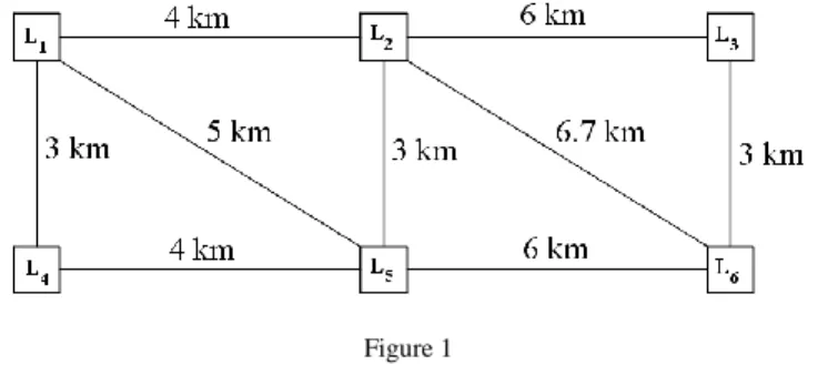
The proposed model can be illustrated by the following simple setting. Let the assumption be that there are 6 locations with distances as in Figure 1 and two facilities to be located. Now, the set of locations is 𝑋 = {𝐿1, … , 𝐿6} and set of facilities is 𝑌 = {𝑌𝑎, 𝑌𝑏}. However, since facilities will be positioned on certain locations, the notation will be 𝑌 = {𝑌𝑎𝑗, 𝑌𝑏𝑘} where {𝑗, 𝑘} ⊂ {1,2, . . . ,6} depends on the intended position of a facility.
Let the assumption be that two layouts are under the consideration:
A: 𝑌 = {𝑌𝑎1, 𝑌𝑏6}, B: 𝑌 = {𝑌𝑎2, 𝑌𝑏5},
i.e., facilities 𝑌𝑎and 𝑌𝑏 are located on locations 𝐿1 and 𝐿6, and 𝐿2 and 𝐿5, respectively. The first calculation is the implementation of the classical case, the second one is done via fuzzy numbers, while the third one is based on the model proposed in this paper. Since the quality (or influence) of facilities in question is the same for the first two approaches (given by examples 4.1 and 4.2), for the sake of simplicity, the following notations will be used:
A: 𝑌 = {𝑌1, 𝑌6}, B: 𝑌 = {𝑌2, 𝑌5},
which is the standard in MCLP problems. However, for the third approach, the quality of facility is relevant and this more complex notation will be used.
Example 4.1 First, a classical MCLP problem without any fuzzy coverage will be used. Let it be supposed that the coverage radius is 5 km, i.e., the function is defined in the following way
𝑓𝐿𝑖(𝐿𝑗) = {1, 𝑖𝑓 d(𝐿𝑖, 𝐿𝑗) ≤ 5 𝑘𝑚, 0, 𝑜𝑡ℎ𝑒𝑟𝑤𝑖𝑠𝑒.
If the facilities are located in 𝐿1 and 𝐿6 then all six locations are covered. On the other hand, if the facilities are located in 𝐿2 and 𝐿5, only four locations are covered, the locations 𝐿3 and 𝐿6 are not covered by this solution. Therefore, the optimal solution is option A.
Figure 1 Location setting
Example 4.2 It will now be supposed that the location can be partially covered, i.e., FMCLP will be considered. The coverage radius for this approach is defined by the following function (see [21])
𝑓𝐿𝑖(𝐿𝑗) = {
1, 𝑖𝑓 d(𝐿𝑖, 𝐿𝑗) ≤ 3𝑘𝑚,
−1
4d(𝐿𝑖, 𝐿𝑗) +7
4, 3 𝑘𝑚 < d(𝐿𝑖, 𝐿𝑗) ≤ 7𝑘𝑚, 0, 𝑜𝑡ℎ𝑒𝑟𝑤𝑖𝑠𝑒.
For option A, the facilities are located in 𝐿1 and 𝐿6 and they are marked as 𝑌1 and 𝑌6 and
𝑓𝐿1: {𝑌1, 𝑌6} → {𝜔1,1, 𝜔1,2}, 𝑓𝐿1(𝑌1) = 1, 𝑓𝐿1(𝑌6) = 0;
𝑓𝐿2: {𝑌1, 𝑌6} → {𝜔2,1, 𝜔2,2}, 𝑓𝐿2(𝑌1) = 0.75, 𝑓𝐿2(𝑌6) = 0.075;
𝑓𝐿3: {𝑌1, 𝑌6} → {𝜔3,1, 𝜔3,2}, 𝑓𝐿3(𝑌1) = 0, 𝑓𝐿3(𝑌6) = 1;
𝑓𝐿4: {𝑌1, 𝑌6} → {𝜔4,1, 𝜔4,2}, 𝑓𝐿4(𝑌1) = 1, 𝑓𝐿4(𝑌6) = 0;
𝑓𝐿5: {𝑌1, 𝑌6} → {𝜔5,1, 𝜔5,2}, 𝑓𝐿5(𝑌1) = 0.5, 𝑓𝐿5(𝑌6) = 0.25;
𝑓𝐿6: {𝑌1, 𝑌6} → {𝜔6,1, 𝜔6,2}, 𝑓𝐿6(𝑌1) = 0, 𝑓𝐿6(𝑌6) = 1.
Therefore, the coverage of location 𝐿1 is max(1,0) = 1, for 𝐿2 is max(0.75,0.075) = 0.75, 𝐿3 is 1, 𝐿4 is 1, 𝐿5 is 0.5 and 𝐿6 is 1. Now, the coverage degree of the option A is
𝑔(𝐴) = 1 + 0.75 + 1 + 1 + 0.5 + 1 = 5.25.
For layout B the following holds
𝑓𝐿1: {𝑌2, 𝑌5} → {𝜔1,1, 𝜔1,2}, 𝑓𝐿1(𝑌2) = 0.75, 𝑓𝐿1(𝑌5) = 0.5;
𝑓𝐿2: {𝑌2, 𝑌5} → {𝜔2,1, 𝜔2,2}, 𝑓𝐿2(𝑌2) = 1, 𝑓𝐿2(𝑌5) = 1;
𝑓𝐿3: {𝑌2, 𝑌5} → {𝜔3,1, 𝜔3,2}, 𝑓𝐿3(𝑌2) = 0.25, 𝑓𝐿3(𝑌5) = 0.075;
𝑓𝐿4: {𝑌2, 𝑌5} → {𝜔4,1, 𝜔4,2}, 𝑓𝐿4(𝑌2) = 0.5, 𝑓𝐿4(𝑌5) = 0.75;
𝑓𝐿5: {𝑌2, 𝑌5} → {𝜔5,1, 𝜔5,2}, 𝑓𝐿5(𝑌2) = 1, 𝑓𝐿5(𝑌5) = 1;
𝑓𝐿6: {𝑌2, 𝑌5} → {𝜔6,1, 𝜔6,2}, 𝑓𝐿6(𝑌2) = 0.075, 𝑓𝐿6(𝑌5) = 0.25.
and
𝑔(𝐵) = 0.75 + 1 + 0.25 + 0.75 + 1 + 0.25 = 4.
Again, layout A is optimal.
The following example illustrates the proposed model based on the Choquet integral. In this case, the quality of facilities, at least the Decision Maker’s perception of that quality, influences the result.
Example 4.3 Let one consider option A. The values that describe the quality of each facility are 𝜇({𝑌𝑎1}) 𝑎𝑛𝑑 𝜇({𝑌𝑏6}), and they are provided by a Decision Maker. Their joint quality, i.e., the measure of how much they complement each other is 𝜇({𝑌𝑎1, 𝑌𝑏6}), can be obtained, as presented in Example 3.1. It is assumed that the measure of an empty set is zero.
The next step is the calculation of the Choquet integral for each function according to the measure µ. That is ”coverage of the location 𝐿𝑖”:
(𝐶) ∫ 𝑓𝐿1d𝜇 = (1 − 0) ∙ 𝜇({𝑦|𝑓𝐿1≥ 1}) = 𝜇({𝑌𝑎1}),
(𝐶) ∫ 𝑓𝐿2d𝜇 = (0.075 − 0) ∙ 𝜇({𝑦|𝑓𝐿2≥ 0.075}) + (0.75 − 0.075) ∙ 𝜇({𝑦|𝑓𝐿2≥ 0.08}) = 0.075𝜇({𝑌𝑎1, 𝑌𝑏6}) + 0.675𝜇({𝑌𝑎1}),
(𝐶) ∫ 𝑓𝐿3d𝜇 = (1 − 0) ∙ 𝜇({𝑦|𝑓𝐿3≥ 1}) = 𝜇({𝑌𝑏6}),
(𝐶) ∫ 𝑓𝐿4d𝜇 = (1 − 0) ∙ 𝜇({𝑦|𝑓𝐿4≥ 1}) = 𝜇({𝑌𝑎1}),
(𝐶) ∫ 𝑓𝐿5d𝜇 = (0.25 − 0) ∙ 𝜇({𝑦|𝑓𝐿5 ≥ 0.25}) + (0.5 − 0.25) ∙ 𝜇({𝑦|𝑓𝐿5≥ 0.5}) = 0.25𝜇({𝑌𝑎1, 𝑌𝑏6}) + 0.25𝜇({𝑌𝑎1}),
(𝐶) ∫ 𝑓𝐿6d𝜇 = (1 − 0) ∙ 𝜇({𝑦|𝑓𝐿6≥ 1}) = 𝜇({𝑌𝑏6}).
The coverage degree of the 𝐿1− 𝐿6 layout is given by 𝑔(𝐴) = ∑ (𝐶) ∫ 𝑓𝑖 𝐿𝑖d𝜇=
2.925𝜇({𝑌𝑎1}) + 2𝜇({𝑌𝑏6}) + 0.325𝜇({𝑌𝑎1, 𝑌𝑏6}). (4) Similarly, for layout 𝐿2− 𝐿5, i.e., for option B, the coverage degree is
𝑔(𝐵) = ∑(𝐶) ∫ 𝑓𝐿𝑖d𝜇
= 0.425(𝜇({𝑌𝑎2}) + 𝜇({𝑌𝑖 𝑏5})) + 3.15𝜇({𝑌𝑎2, 𝑌𝑏5}). (5)
Let it be assumed that the qualities of two facilities in question are graded with, e.g., 0.6 and 0.8 and if overlaps are negligible, the 𝑆𝐿 can be used as the aggregation operator. For option A, if the facility of quality 0.6 is placed on location 𝐿1, the following holds
𝜇({𝑌𝑎1}) = 0.6, 𝜇({𝑌𝑏6}) = 0.8, 𝜇({𝑌𝑎1, 𝑌𝑏6}) = 1 and g(A)=3.68.
On the other hand, for option B, if the facility of quality 0.6 is placed on location 𝐿2, the following holds
𝜇({𝑌𝑎2}) = 0.6, 𝜇({𝑌𝑏5}) = 0.8, 𝜇({𝑌𝑎2, 𝑌𝑏5}) = 1 and g(B)=3.745.
Now, since the quality of facilities is taken into account, the result is different and the optimal solution is layout B.
While in MCLP and FMCLP the quality of facilities is not taken in to consideration, it has a high influence on the result in the proposed model. The flexibility of the proposed model can be additionally illustrated by the following example, that is the continuation of the previous one.
Example 4.4 If the positions of facilities in option A are inverted, i.e., if the layout is A: 𝑌 = {𝑌𝑏1, 𝑌𝑎6}, the following holds
𝜇({𝑌𝑏1}) = 0.8, 𝜇({𝑌𝑎6}) = 0.6, 𝜇({𝑌𝑏1, 𝑌𝑎6}) = 1 and g(A)=3.865.
That is, now this layout is better than layout B.
Remark 4.4 If the assumption is that all facilities are of the same quality, e.g., quality 1, the proposed model coincides with FMCLP.
As seen from the previous examples, the new model allows the quality of facilities, given by the measure µ, to influence the final decision. All four examples are summarized in Table 1. The optimal option is marked with *.
Table 1
Comparison of coverage degrees
MCLP FMCLP MODEL Ch, I MODEL Ch, II
option A 6* 5.24* 3.68 3.865*
option B 4 4 3.745* 3.745
Remark 4.5 If there is no other facility (e.g. hospital) near 𝑌1 (𝐿1− 𝐿6 layout), as illustrated in the previous example, the coverage degree of the location 𝐿1 where is located 𝑌1 corresponds to 𝜇({𝑌1}), more precisely, it corresponds to the quality of 𝑌1. On the other hand, if the layout 𝐿2− 𝐿5 is observed, hospitals are close, thus the coverage of the location 𝐿2 corresponds to 𝜇({𝑌2, 𝑌5}), i.e., to the joint measure of facilities 𝑌2 and 𝑌5.
Conclusion
This paper presents a generalization of the MCLP obtained by the incorporation of the Choquet integral into FMCLP. The nature of the observed integral takes into consideration the joint influence of each facility combination, which has not been done in any type of location problem before. The introduction of fuzzy integrals into the FMLCP makes the model more flexible and adaptable to real life problems. As it can be seen from (4), expert opinion of a Decision Maker given through set-function µ has a direct influence on the result. Thus a practical need for a new type of location problem is justified, and will further be called Extended FMCLP.
Acknowledgement
The authors would like to thank Humberto Bustince for providing the idea to use fuzzy integrals in FMCLP. This was suggested during a discussion at the FSTA 2014 conference.
This work was supported by the Ministry of Science and Technological Development of Republic of Serbia.
References
[1] V. Batanovic, D. Petrovic, R. Petrovic: Fuzzy Logic-based Algorithms for Maximum Covering Location Problems, Information Sciences 179 (1-2) (2009) 120-129, DOI: 10.1016/j.ins.2008.08.019
[2] P. Benvenuti, and R. Mesiar: ”Integrals with Respect to a General Fuzzy Measure”, Fuzzy Measures and Integrals (M. Grabisch, T. Murofushi, M.
Sugeno eds.) Physica-Verlag (Springer-Verlag Company), Heidelberg 2000, 205-232
[3] P. Benvenuti, R. Mesiar, D. Vivina: ”Monotone Set Functions-based Integrals”, Handbook of Measure Theory (E. Pap ed.), Elsevier, Amsterdam, 2002, 1329-1379
[4] G. Choquet, ”Theory of Capacities”: Annales de l’Institut Fourier 5 (1953), 131-295
[5] R. Church and C. ReVelle: Maximal Covering Location Problem, Papers of the Regional Science Association 32 (1974) 101-118
[6] R. Church: The Planar Maximal Covering Location Problem, Journal of Regional Science 2(24) (1984) 185-201
[7] J. R. Current and J. E. Storbeck: Capacitated Covering Models, Environment and Planning B: Planning and Design 15(2) (1988) 153-163 [8] J. Darzentas: A Discrete Location Model with Fuzzy Accessibility
Measures, Fuzzy Sets and Systems 23 (1987) 149-154, DOI: 10.1016/0165- 0114(87)90106-0
[9] S. Davari, M. H. F. Zarandi, A. Hemmati: Maximal Covering Location Problem (MCLP) with Fuzzy Travel Times, Expert Systems with Applications 38 (12) (2011) 14535-14541, DOI:
10.1016/j.eswa.2011.05.031
[10] D. Deneberg: Non-Additive Measure and Integral, Kluwer Academic Publishers, Dordrecht-Boston-London, 1994
[11] M. Detyniecki: Fundamentals on Aggregation operators, http://www.cs.berkeley.edu/˜marcin/agop.pdf
[12] R. Z. Farahani, N. Asgari, N. Heidari, M. Hosseininia, M. Goh: Covering Problems in Facility Location: A Review, Computers and Industrial Engineering 62 (2012) 368-407, DOI:10.1016/j.cie.2011.08.020
[13] M. Grabisch: k-additive Fuzzy Measures, 6th International Conference on Information Processing and Management of Uncertainty in Knowledge- Based Systems (IPMU), Granada, Spain, July 1996
[14] M. Grabisch, J. Marichal, R. Mesiar, and E. Pap: Aggregations Functions, Cambridge University Press, 2009
[15] M. Grabisch, H.T. Nguyen, and E.A. Walker: Fundamentals of Uncertainty Calculi with Applications to Fuzzy Inference, Kluwer Academics Publishers, Dordrecht, 1995
[16] E. P. Klement, R. Mesiar and E. Pap: Triangular Norms, Series: Trends in Logic, Kluwer Academic Publishers, Vol. 8, Dordrecht 2000
[17] A. T. Murray, D. Tong, and K. Kim: Enhancing Classic Coverage Location Models, International Regional Science Review 33(2) (2010) 115-133, DOI: 10.1177/0160017609340149
[18] E. Pap: Null-Additive Set Functions, Kluwer Academic Publishers, Dordrecht, 1995
[19] J. A. M. Perez, J. M. M. Vega, J. L. Verdegay: Fuzzy Location Problems on Networks, Fuzzy Sets and Systems 142 (2004) 393-405, DOI:
10.1016/S0165- 0114(03)00091-5
[20] C. ReVelle, and K. Hogan: The Maximum Availability Location Problem, Transportation Science 23 (1989) 192-200
[21] A. Takaci, M. Maric, D. Drakulic: The Role of Fuzzy Sets in Improving Maximal Covering Location Problem (MCLP). Procc. of SISY 2012, Subotica, Serbia 103-106
[22] Z. Wang, and G. J. Klir: Generalized Measure Theory, Springer, 2000 [23] R. R. Yager: ”On Ordered Weighted Averaging Aggregation Operators in
Multicriteria Decision Making,” IEEE Transactions on Systems, Man and Cybernetics 18(1988), 183-190