Rectifiability of orbits for two-dimensional nonautonomous differential systems
Dedicated to Professor Hiroyuki Usami on the occasion of his sixtieth birthday
Masakazu Onitsuka
B1and Satoshi Tanaka
*21Department of Applied Mathematics, Okayama University of Science, Ridai-cho 1–1, Okayama 700–0005, Japan
2Mathematical Institute, Tohoku University, Aoba 6–3, Aramaki, Aoba-ku, Sendai 980–8578, Japan
Received 28 September 2020, appeared 24 March 2021 Communicated by Mihály Pituk
Abstract. The present study is concerned with the rectifiability of orbits for the two- dimensional nonautonomous differential systems. Criteria are given whether the orbit has a finite length (rectifiable) or not (nonrectifiable). The global attractivity of the zero solution is also discussed. In the linear case, a necessary and sufficient condition can be obtained. Some examples and numerical simulations are presented to explain the results.
Keywords: rectifiability, global attractivity, two-dimensional nonautonomous system.
2020 Mathematics Subject Classification: 34A34, 34D20, 26B15.
1 Introduction
We consider the two-dimensional nonautonomous differential system x0 = −e(t)x+ f(t)y−p(t)x x2+y2λ
, y0 = −g(t)x−h(t)y−q(t)y x2+y2λ
,
(1.1) wheree, f,g,h, pandqare continuous fort≥ t0, andλ>0. Since the right hand side of this system is continuously differentiable with respect to(x,y), so it satisfies the Lipschitz condi- tion. Therefore, the local existence and uniqueness of solutions of (1.1) are guaranteed for the initial-value problem. We can show that, for each t0 ∈ R and(x0,y0) ∈ R2, the initial value problem (1.1) with (x(t0),y(t0)) = (x0,y0) has a unique solution on[t0,∞) under some con- ditions (this fact will be shown in Lemma3.4.). We denote it by(x(t;t0,x0,y0),y(t;t0,x0,y0)). Clearly, (1.1) has the zero solution(x(t),y(t))≡(0, 0). Throughout this paper,k(x,y)kmeans
BCorresponding author. Email: onitsuka@xmath.ous.ac.jp
*Email: satoshi.tanaka.d4@tohoku.ac.jp
the Euclidean norm of(x,y); that is,k(x,y)k:= px2+y2. Here, let us give a definition about the zero solution of (1.1). The zero solution of (1.1) is said to beglobally attractiveif
tlim→∞k(x(t;t1,x0,y0),y(t;t1,x0,y0))k=0
for any t1 ∈ [t0,∞) and any (x0,y0) ∈ R2. Now rewrite (x(t;t0,x0,y0),y(t;t0,x0,y0)) by (x(t),y(t)). We define theorbitof(x(t),y(t))by
Γ(t0,x,y):={(x(t),y(t))∈R2:t≥ t0}.
The orbitΓ(t0,x,y)is said to besimpleif(x(t1),y(t1))6= (x(t2),y(t2))for anyt1,t2∈ [t0,∞)with t1 6= t2. Now, we assume that the zero solution of (1.1) is globally attractive. The simple orbit Γ(t0,x,y)is said to berectifiableif the length ofΓ(t0,x,y)is finite, that is,
tlim→∞ Z t
t0
k(x0(s),y0(s))kds<∞.
Otherwise, it is said to benonrectifiable.
When λ= 1 and e(t) =h(t) = a0, f(t) =g(t) =1, p(t) =q(t) =1 for all t ≥ t0, system (1.1) reduces to the planar nonlinear differential system
x0 =y−x x2+y2+a0 , y0 =−x−y x2+y2+a0
. (1.2)
For every solution (x(t),y(t))of (1.2), using the polar coordinate transformation x = rcosθ, y=rsinθ, then we have
r0 = −r r2+a0 , θ0 = −1.
Fromθ0 = −1, every orbitΓ(t0,x,y)of (1.2) is rotating in a clockwise direction. Moreover, if we supposea0 ≥0, thenr0 ≤ −r3, so that
r(t)≤ p 1
2(t−t0) +r−2(t0) ≤ p 1 2(t−t0)
fort ≥ t0. This says that a0 ≥ 0 implies that the zero solution of (1.2) is globally attractive.
Hence, every orbitΓ(t0,x,y)of (1.2) is a spiral.
Remark 1.1. Since (1.2) is an autonomous system andr0 ≤ −r3, the orbitΓ(t0,x,y)corresponding to any nontrivial solution(x(t),y(t))of (1.2) is simple.
Miliši´c, Žubrini´c and Županovi´c [10] studied rectifiability for more general autonomous differential systems based on planar system (1.2). Theorem 8 given in [10] and the above mentioned facts imply the following.
Theorem A. Let(x(t),y(t)) be any nontrivial solution of (1.2). Suppose that a0 ≥ 0 holds. Then the zero solution of (1.2)is globally attractive, the orbitΓ(t0,x,y)corresponding to(x(t),y(t))is simple, and (i) and (ii) below hold:
(i) if a0 >0, then the orbitΓ(t0,x,y) is rectifiable;
(ii) if a0 =0, then the orbitΓ(t0,x,y) is nonrectifiable.
Remark 1.2. Miliši´c, Žubrini´c and Županovi´c [10] and Žubrini´c and Županovi´c [23,24] dealt with the rectifiability and the fractal analysis of spiral orbits (or trajectories) of some au- tonomous systems including (1.2). They dealt with more general, but autonomous systems.
This study focuses on the rectifiability of the nonautonomous systems.
For simplicity, we denote
α1(t):=min{e(t),h(t)} − |f(t)−g(t)|
2 , β1(t):=min{p(t),q(t)}, α2(t):=max{e(t),h(t)}+|f(t)−g(t)|
2 , β2(t):=max{p(t),q(t)},
(1.3)
and
γ1(t):=−max{f(t),g(t)} −|e(t)−h(t)|
2 − |p(t)−q(t)|
2 ,
γ2(t):=−min{f(t),g(t)}+ |e(t)−h(t)|
2 +|p(t)−q(t)|
2 .
(1.4)
Ife(t)≡ h(t), f(t)≡g(t)and p(t)≡q(t), then
α1(t) =α2(t) =e(t), β1(t) = β2(t) =p(t) and γ1(t) =γ2(t) =−f(t) fort ≥t0. Moreover, for eachc>0, we denote
ρi(t;c):=exp
2λ Z t
t0
αi(s)ds c+2λ Z t
t0
βi(s)exp
−2λ Z s
t0
αi(τ)dτ
ds
, i=1, 2. (1.5) The first main result in this paper is as follows.
Theorem 1.3. Let(x(t),y(t))be any nontrivial solution of (1.1). Suppose that
α1(t)≥0, β1(t)≥0 for t≥t0, (1.6) α1(t) +β1(t)>0 for t≥t0, (1.7) and
tlim→∞ Z t
t0
α1(s)ds= ∞ or lim
t→∞ Z t
t0
β1(s)ds=∞. (1.8)
Then the zero solution of (1.1) is globally attractive, the orbitΓ(t0,x,y) corresponding to (x(t),y(t))is simple, and (i), (ii) and (iii) below hold:
(i) ifα1(t)>0for t≥ t0, and
lim sup
t→∞
max{|γ1(t)|,|γ2(t)|}
α1(t) <∞, (1.9)
then the orbitΓ(t0,x,y) is rectifiable;
(ii) if0<λ<1/2and
lim sup
t→∞
max{|γ1(t)|,|γ2(t)|}
α1(t)ρ1(t;c) +β1(t) <∞ for each c>0, (1.10) then the orbitΓ(t0,x,y) is rectifiable;
(iii) ifλ≥1/2and
lim inf
t→∞
max{γ1(t),−γ2(t), 0}
α2(t)ρ2(t;c) +β2(t) >0 for each c >0, (1.11) then the orbitΓ(t0,x,y)is nonrectifiable.
Using Theorem1.3we get the following result, immediately.
Corollary 1.4. Let(x(t),y(t))be any nontrivial solution of (1.1). Let(x(t),y(t))be any nontrivial solution of (1.1). Suppose that(1.6), (1.7) and(1.8)hold. Then the zero solution of (1.1)is globally attractive, the orbitΓ(t0,x,y)corresponding to(x(t),y(t))is simple, and (i), (ii) and (iii) below hold:
(i) ifα1(t)>0for t ≥t0, and(1.9), then the orbitΓ(t0,x,y)is rectifiable;
(ii) if0<λ<1/2andβ1(t)>0for t≥t0, and lim sup
t→∞
max{|γ1(t)|,|γ2(t)|}
β1(t) < ∞, (1.12)
then the orbitΓ(t0,x,y)is rectifiable;
(iii) ifλ≥1/2andα2(t) =0for t≥t0, and lim inf
t→∞
max{γ1(t),−γ2(t), 0}
β2(t) >0, (1.13)
then the orbitΓ(t0,x,y)is nonrectifiable.
Corollary1.4is expressed in a form which does not include the functionsρ1andρ2. If e(t) = h(t) = a0 ≥ 0, f(t) = g(t) = 1, p(t) = q(t) = 1 for all t ≥ t0, then system (1.1) reduces to the planar system
x0 =−a0x+y−x x2+y2λ
, y0 =−x−a0y−y x2+y2λ.
(1.14) In this case, we know thatα1(t) =α2(t) = a0, β1(t) = β2(t) =1 and γ1(t) =γ2(t) =−1 for allt≥t0. Then (1.6), (1.7), (1.8), (1.12) and (1.13) hold. Ifa0>0 then (i) in Corollary1.4holds.
Hence, we get the following result, immediately.
Corollary 1.5. Let (x(t),y(t)) be any nontrivial solution of (1.14). Suppose that a0 ≥ 0 holds.
Then the zero solution of (1.14)is globally attractive, the orbitΓ(t0,x,y)corresponding to(x(t),y(t))is simple, and (i), (ii) and (iii) below hold:
(i) if a0 >0, then the orbitΓ(t0,x,y) is rectifiable;
(ii) if a0 =0and0< λ<1/2, then the orbitΓ(t0,x,y)is rectifiable;
(iii) if a0 =0andλ≥1/2, then the orbitΓ(t0,x,y)is nonrectifiable.
Remark 1.6. From Corollary1.5, TheoremAis easily obtained.
Figures 1.1–1.4 below show that the orbits corresponding to the nontrivial solution (x(t),y(t)) of (1.14) with (x(0),y(0)) = (0.9, 0). We choose a0 and λ as follows: a0 = 0.1 andλ=1 in Fig. 1.1; a0=0 andλ=0.1 in Fig. 1.2; a0 =0 andλ=0.5 in Fig.1.3;a0=0 and λ=0.9 in Fig.1.4.
-0.5 0.5 1.0 x
-0.8 -0.6 -0.4 -0.2 0.2 0.4 0.6
Figure 1.1: a0 = 0.1,λ = 1; rectifi- able.
-0.5 0.5 1.0 x
-0.8 -0.6 -0.4 -0.2 0.2 0.4 0.6
Figure 1.2: a0 = 0, λ = 0.1; rectifi- able.
-0.5 0.5 1.0 x
-0.8 -0.6 -0.4 -0.2 0.2 0.4 0.6
Figure 1.3: a0 =0,λ=0.5; nonrec- tifiable.
-0.5 0.5 1.0 x
-0.8 -0.6 -0.4 -0.2 0.2 0.4 0.6
Figure 1.4: a0=0, λ=0.9; nonrec- tifiable.
The second main result in this paper is as follows.
Theorem 1.7. Let (x(t),y(t)) be any nontrivial solution of (1.1). Suppose that (1.6), (1.7) and (1.8) hold. Then the zero solution of (1.1) is globally attractive, the orbit Γ(t0,x,y) corresponding to (x(t),y(t))is simple, and (i) and (ii) below hold:
(i) if
tlim→∞
Z t
t0
q
[α2(s) +β2(s)(ρ1(s;c))−1]2+ (max{|γ1(s)|,|γ2(s)|})2 (ρ1(s;c))2λ1 ds
< ∞ (1.15) for each c>0, then the orbitΓ(t0,x,y)is rectifiable;
(ii) if
tlim→∞ Z t
t0
q
[α1(s) +β1(s)(ρ2(s;c))−1]2+ (max{γ1(s),−γ2(s), 0})2
(ρ2(s;c))2λ1 ds= ∞ (1.16) for each c>0, then the orbitΓ(t0,x,y)is nonrectifiable.
If p(t) ≡ q(t) ≡ 0, then system (1.1) reduces to the two-dimensional linear differential system
x0 = −e(t)x+ f(t)y,
y0 = −g(t)x−h(t)y. (1.17)
Note thatβ1(t)≡ β2(t)≡0. For this linear system, using Theorem1.7, we obtain the following corollary.
Corollary 1.8. Let(x(t),y(t))be any nontrivial solution of (1.17). Suppose that α1(t)>0 for t≥t0,
and
tlim→∞ Z t
t0
α1(s)ds= ∞.
Then the zero solution of (1.17)is globally attractive, the orbitΓ(t0,x,y)corresponding to(x(t),y(t))is simple, and (i) and (ii) below hold:
(i) if
tlim→∞ Z t
t0
q
α22(s) + (max{|γ1(s)|,|γ2(s)|})2exp
−
Z s
t0
α1(τ)dτ
ds<∞, then the orbitΓ(t0,x,y)is rectifiable;
(ii) if
tlim→∞ Z t
t0
q
α21(s) + (max{γ1(s),−γ2(s), 0})2exp
−
Z s
t0
α2(τ)dτ
ds=∞, then the orbitΓ(t0,x,y)is nonrectifiable.
In particular, if e(t)≡ h(t), f(t)≡ g(t)then we have the two-dimensional linear differen- tial system
x0 =−e(t)x+ f(t)y,
y0 =−f(t)x−e(t)y. (1.18)
In this case, we know thatα1(t)≡ α2(t)≡ e(t), β1(t)≡β2(t)≡ 0 andγ1(t)≡γ2(t)≡ −f(t). We can establish the following result by Corollary1.8.
Corollary 1.9. Let(x(t),y(t))be any nontrivial solution of (1.18). Suppose that
e(t)>0 for t≥ t0, (1.19)
and
tlim→∞ Z t
t0
e(s)ds= ∞. (1.20)
Then the zero solution of (1.18)is attractive, the orbitΓ(t0,x,y)corresponding to (x(t),y(t))is simple, and the orbitΓ(t0,x,y)is rectifiable if and only if
tlim→∞ Z t
t0
q
e2(s) + f2(s)exp
−
Z s
t0
e(τ)dτ
ds<∞. (1.21)
Remark 1.10. It is well known that the local attractivity and the global attractivity are equiv- alent in the linear case (see [1,20–22]). Hence, the attractivity of (1.18) means the global attractivity.
Consider the two-dimensional nonautonomous linear system x0 =−1
tx+tσy, y0 =−tσx−1
ty,
(1.22)
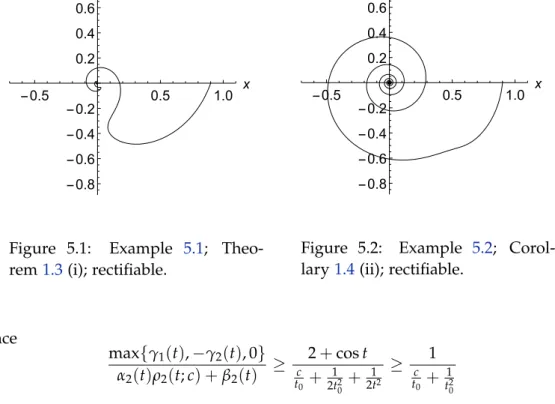
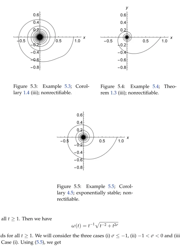
where σ ∈ R and t ≥ 1. Then assumptions (1.19) and (1.20) are easily satisfied. By Corol- lary1.9, the zero solution of (1.22) is attractive, the orbitΓ(t0,x,y) corresponding to (x(t),y(t)) is simple. Moreover, we can see that the orbit Γ(t0,x,y) is rectifiable if and only if σ < 0 (The conditions of Corollary1.9will be confirmed in Section 5).
Remark 1.11. Our result on the rectifiability of orbits (or trajectories) of (1.22) is the same as one that the special case of the result given by Naito, Paši´c and Tanaka [12, Example 5.2].
Note here that they dealt with half-linear systems. On the other hand, as related research, the rectifiability results of the authors [13,14] can be mentioned, but note that this study has no inclusion relation with them. Moreover, we can find many results on the rectifiability and the fractal analysis of the systems and equations. For example, the reader is referred to [4–7,9,11,15–19].
In the next section, we will discuss the rectifiability for more general systems under the assumption that the zero solution is globally attractive, and the orbit Γ(t0,x,y) is simple. In Section 3, the simplicity and the global attractivity for (1.1) are considered. In Section 4, we prove Theorems 1.3 and 1.7. In Section 5, some examples and numerical simulations are presented.
2 Rectifiability
In this section, we consider the two-dimensional nonautonomous differential system x0 = F1(t,x,y),
y0 = F2(t,x,y), (2.1)
where F1andF2are continuously differentiable with respect to(x,y), and satisfying (F1(t, 0, 0),F2(t, 0, 0))≡(0, 0).
For every solution (x(t),y(t)) of (2.1), we introduce the polar coordinate transformation x=rcosθ,y=rsinθ. Then we obtain
r0 =G1(t,r,θ),
rθ0 =G2(t,r,θ), (2.2)
where G1 andG2 are defined by
G1(t,r,θ) =cosθF1(t,rcosθ,rsinθ) +sinθF2(t,rcosθ,rsinθ) (2.3) and
G2(t,r,θ) =cosθF2(t,rcosθ,rsinθ)−sinθF1(t,rcosθ,rsinθ). (2.4) The obtained result is as follows.
Theorem 2.1. Let G1and G2be the functions given by(2.3)and(2.4), respectively. Let(x(t),y(t))be any nontrivial solution of (2.1)on[t0,∞). Suppose that the zero solution of (2.1)is globally attractive, and the orbitΓ(t0,x,y)corresponding to(x(t),y(t))is simple. Then, (i) and (ii) below hold:
(i) if there exist an r>0and a continuous function h:(0,r)→(0,∞)such that
k(G1(t,r,θ),G2(t,r,θ))k ≤ −h(r)G1(t,r,θ), (t,r,θ)∈[t0,∞)×(0,r)×R, (2.5) and
rlim→+0
Z r
r h(η)dη<∞, (2.6)
then the orbitΓ(t0,x,y)is rectifiable;
(ii) if there exist an r>0and a continuous function h:(0,r)→(0,∞)such that
k(G1(t,r,θ),G2(t,r,θ))k ≥ −h(r)G1(t,r,θ), (t,r,θ)∈[t0,∞)×(0,r)×R, (2.7) and
rlim→+0
Z r
r h(η)dη=∞, (2.8)
then the orbitΓ(t0,x,y)is nonrectifiable.
Proof. Let(x(t),y(t))be any nontrivial solution of (2.1). Define the functionsr andθ by x(t) =r(t)cosθ(t), y(t) =r(t)sinθ(t)
fort ≥t0, where
r(t) =k(x(t),y(t))k.
Then(r(t),θ(t))is a solution to (2.2). Since the existence and uniqueness of solutions of (2.1) are guaranteed for the initial-value problem, the zero solution(x(t),y(t)) ≡ (0, 0) is unique.
Thus, r(t) > 0 for t ≥ t0. This together with the global attractivity of (2.1) implies that limt→∞r(t) =0, and there exists a T>0 such that
r(t)∈(0,r) (2.9)
fort ≥t0+T.
Now, we consider case (i). Using (2.5) and (2.9), we have
k(x0(t),y0(t))k= k(F1(t,x(t),y(t)),F2(t,x(t),y(t)))k
= q
(cosθF1+sinθF2)2+ (cosθF2−sinθF1)2
= k(G1(t,r(t),θ(t)),G2(t,r(t),θ(t)))k
≤ −h(r(t))G1(t,r(t),θ(t)) =−h(r(t))r0(t)
fort ≥ t0+T. Since h(r)is a positive continuous function on (0,r), and (2.9) holds, we see that
Z t
t0+T
k(x0(s),y0(s))kds≤ −
Z t
t0+T
h(r(s))r0(s)ds=
Z r(t0+T)
r(t)
h(η)dη
≤
Z r
r(t)
h(η)dη
fort ≥t0+T. Therefore, we have Z t
t0
k(x0(s),y0(s))kds=
Z t0+T t0
k(x0(s),y0(s))kds+
Z t
t0+T
k(x0(s),y0(s))kds
≤
Z t0+T t0
k(x0(s),y0(s))kds+
Z r
r(t)h(η)dη fort ≥t0+T. Using (2.6), (2.9) with limt→∞r(t) =0, we conclude that
tlim→∞ Z t
t0
k(x0(s),y0(s))kds< ∞.
Hence, the simple orbit Γ(t0,x,y) is rectifiable.
Next, we consider case (ii). From (2.7) and (2.9), we have
k(x0(t),y0(t))k ≥ −h(r(t))G1(t,r(t),θ(t)) =−h(r(t))r0(t)
for t ≥ t0+T. Sinceh(r)is a positive continuous function on (0,r), and (2.9) holds, we see that
Z t
t0
k(x0(s),y0(s))kds≥
Z t
t0+T
k(x0(s),y0(s))kds
≥ −
Z t
t0+Th(r(s))r0(s)ds=
Z r(t0+T)
r(t) h(η)dη
=
Z r
r(t)h(η)dη−
Z r
r(t0+T)h(η)dη fort ≥t0+T. From (2.8), (2.9) with limt→∞r(t) =0, we get
tlim→∞ Z t
t0
k(x0(s),y0(s))kds= ∞.
Consequently, the simple orbitΓ(t0,x,y) is nonrectifiable. This completes the proof.
For our main system (1.1), we find that
F1(t,x,y) =−e(t)x+ f(t)y−p(t)x x2+y2λ
, F2(t,x,y) =−g(t)x−h(t)y−q(t)y x2+y2λ
, and
G1(t,r,θ) =− e(t)cos2θ+h(t)sin2θ
r+ (f(t)−g(t))rsinθcosθ
− p(t)cos2θ+q(t)sin2θ r2λ+1, G2(t,r,θ) =− g(t)cos2θ+ f(t)sin2θ
r+ (e(t)−h(t))rsinθcosθ + (p(t)−q(t))r2λ+1sinθcosθ.
(2.10)
3 Simplicity and global attractivity
In this section, we deal with the simplicity and the global attractivity for our main system (1.1). First, we give two lemmas.
Lemma 3.1. Let G1 be the function given in(2.10). Then
G1(t,r,θ)≤ −α1(t) +β1(t)r2λ r holds for t≥t0and r ∈[0,∞), where α1 andβ1are given in(1.3).
Proof. By (2.10), we get
G1(t,r,θ)≤ −min{e(t),h(t)}r+|f(t)−g(t)|
2 r−min{p(t),q(t)}r2λ+1
=−α1(t) +β1(t)r2λ r fort ≥t0andr∈[0,∞).
Lemma 3.2. Suppose that(1.6)and(1.7)hold. Then
α1(t) +β1(t)r2λ r >0 holds for t≥t0and r ∈(0,∞), whereα1 andβ1are given in(1.3).
Proof. By way of contradiction, we suppose that there exists at1≥ t0 such that
α1(t1) +β1(t1)r2λ r≤0.
From (1.6) andr∈ (0,∞), we have
α1(t1) +β1(t1)r2λ=0.
This together with (1.6) says that α1(t1) = β1(t1) = 0. However, this contradicts assumption (1.7).
We now consider the simplicity of the nontrivial solutions to (1.1). The obtained result is as follows.
Lemma 3.3. Let(x(t),y(t))be a nontrivial solution of (1.1). Suppose that(1.6)and(1.7)hold. Then the orbitΓ(t0,x,y)corresponding to(x(t),y(t))is simple.
Proof. Let(x(t),y(t))be a nontrivial solution of (1.1). Assume to the contrary that there exist t1, t2 ∈ [t0,∞) such that t1 < t2 with (x(t1),y(t1)) = (x(t2),y(t2)). Let (r(t),θ(t)) be the solution of (2.2) with (2.10) corresponding to (x(t),y(t)). Then r(t1) = r(t2) holds. Since (x(t),y(t)) is a nontrivial solution and the zero solution is unique, we know that r(t) > 0 for all t ≥ t0. From Lemmas 3.1 and 3.2, we see that r0(t) < 0 for t ≥ t0. Integrating this inequality fromt1 tot2, we obtain
r(t2)−r(t1) =
Z t2
t1 r0(t)dt<0.
This is a contradiction. Consequently,Γ(t0,x,y)is a simple orbit.
We will give an important inequality.
Lemma 3.4. Let(x(t),y(t))be a nontrivial solution of (1.1)with the initial condition(x(t0),y(t0)) = (x0,y0). Let (r(t),θ(t)) be the solution of (2.2) with (2.10) corresponding to (x(t),y(t)). Suppose that β1(t)≥0holds for t≥t0. Then(x(t),y(t))exists on[t0,∞)and is the unique solution of (1.1) with(x(t0),y(t0)) = (x0,y0), and the inequality
0<r(t)≤exp
−
Z t
t0
α1(s)ds r−2λ(t0) +2λ Z t
t0
β1(s)exp
−2λ Z s
t0
α1(τ)dτ
ds −2λ1
(3.1) holds for t ≥t0, where α1 andβ1are given in(1.3).
Proof. Let (x(t),y(t)) be a nontrivial solution of (1.1) with (x(t0),y(t0)) = (x0,y0). Let (r(t),θ(t)) be the solution of (2.2) with (2.10) corresponding to (x(t),y(t)). Let I ⊂ [t0,∞) be the maximal interval of the existence of(x(t),y(t)). Thenr(t)>0 holds for t∈ I, from the uniqueness of the zero solution. Using Lemma 3.1, we have
r0(t)≤ −α1(t) +β1(t)r2λ(t)r(t)
fort ∈ I. Setz(t):=r−2λ(t). Then, it follows from the above inequality andr(t)>0 that z0(t) =−2λr−2λ−1(t)r0(t)≥2λr−2λ(t)α1(t) +β1(t)r2λ(t)=2λα1(t)z(t) +2λβ1(t) fort ∈ I. Hence
exp
−2λ Z t
t0
α1(s)ds
z(t) 0
≥2λβ1(t)exp
−2λ Z t
t0
α1(s)ds
fort ∈ I. Integrating this inequality fromt0tot, we get exp
−2λ Z t
t0
α1(s)ds
z(t)≥z(t0) +2λ
Z t
t0
β1(s)exp
−2λ Z s
t0
α1(τ)dτ
ds, and so that
r−2λ(t) =z(t)≥exp
2λ Z t
t0
α1(s)ds r−2λ(t0) +2λ Z t
t0
β1(s)exp
−2λ Z s
t0
α1(τ)dτ
ds
fort ∈ I. Therefore, if β1(t)≥0 fort ≥t0, then we obtain (3.1) fort∈ I.
Using the above inequality andβ1(t)≥0 fort≥t0, we have r−2λ(t)≥exp
2λ
Z t
t0
α1(s)ds
r−2λ(t0), and thus,
0<k(x(t),y(t))k ≤ k(x0,y0)kexp
−
Z t
t0
α1(s)ds
for t∈ I. (3.2) This inequality means that I = [t0,∞), that is, any nontrivial solution of (1.1) exists on[t0,∞) by a standard argument of a general theory on ordinary differential equations. Consequently, the initial value problem (1.1) with(x(t0),y(t0)) = (x0,y0)has a unique solution on[t0,∞).
Next, we consider the global attractivity for (1.1). Assuming a stronger condition, we can get stronger stability. The zero solution is said to be globally exponentially stableif there exists a k > 0 and, for any η > 0, there exists a δ(η) > 0 such that t1 ∈ R with t1 ≥ t0 and k(x0,y0)k<ηimply
k(x(t;t1,x0,y0),y(t;t1,x0,y0))k ≤δ(η)k(x0,y0)ke−k(t−t1) for all t≥t1. The following lemma is established.
Lemma 3.5. Suppose that (1.6) and (1.8) hold, where α1 and β1 are given in (1.3). Then the zero solution of (1.1)is globally attractive. In particular, if there exists an a>0such that
α1(s)≥a for t≥t0, (3.3)
then the zero solution of (1.1)is globally exponentially stable.
Proof. Lett1satisfyt1≥ t0. Let(x(t),y(t))be any nontrivial solution of (1.1) with(x(t1),y(t1))
= (x0,y0). Let (r(t),θ(t)) be the solution of (2.2) with (2.10) corresponding to (x(t),y(t)). Using Lemma3.4, we have inequality (3.1) fort ≥t1.
Now we consider the case limt→∞Rt
t0α1(s)ds<∞. This together with (1.8) yields
tlim→∞ Z t
t0
β1(s)ds=∞.
LetL:=limt→∞Rt
t0α1(s)ds≥0. Using this and (3.1), we obtain 0<k(x(t),y(t))k=r(t)≤ 1
r−2λ(t1) +2λe−2λLRt
t1β1(s)ds2λ1
< 1
2λe−2λLRt
t1β1(s)ds2λ1 fort ≥ t1. Hence, any nontrivial solution of (1.1) tends to (0, 0)as t → ∞. That is, the zero solution of (1.1) is globally attractive.
Next we consider the case limt→∞Rt
t0α1(s)ds = ∞. Then, by assumption (1.6), we obtain inequality (3.2). Therefore, the zero solution of (1.1) is globally attractive. Moreover, if we sup- pose condition (3.3), then inequality (3.2) implies global exponential stability. This completes the proof.
Remark 3.6. Ifα1(t)≡0 then, it does not imply the (global) exponential stability for (1.1). For example, we consider the caseλ=1,e(t) =h(t) =0 and f(t) = g(t) =1 andp(t) =q(t) =1 fort ≥ t0. That is, α1(t) = α2(t) = 0, β1(t) = β2(t) = 1 and γ1(t) = γ2(t) = −1 fort ≥ t0. From (2.2) and (2.10), we have
r0 =−r3. Solving this equation, we get
r(t) = p 1
2(t−t0) +r−2(t0)
fort ≥ t0. Thus, the zero solution is not exponentially stable. Although not described here in detail, we can see that the zero solution of this system is uniformly asymptotically stable.
It is well known that the exponential stability implies the uniform asymptotic stability; the uniform asymptotic stability implies the asymptotic stability (the zero solution is attractive and stable). If (1.1) is a periodic or autonomous system, then the asymptotic stability and the uniform asymptotic stability are equivalent. For example, see [2,3,8,21,22]. Moreover, if (1.1) is a linear system, the uniform asymptotic stability and the exponential stability are equivalent. For example, the reader is referred to [3,21,22] and the references cited therein. In general, our main equations are nonautonomous and nonlinear, so their stabilities are often different.
4 Proofs of the main theorems
Before proving the main theorems, we give three lemmas.
Lemma 4.1. Let G1be the function given in(2.10). Then
G1(t,r,θ)≥ −α2(t) +β2(t)r2λ
r (4.1)
holds for t ≥t0and r∈ [0,∞), whereα2andβ2are given in(1.3).
Proof. By (2.10), we get
G1(t,r,θ)≥ −max{e(t),h(t)}r−|f(t)−g(t)|
2 r−max{p(t),q(t)}r2λ+1
=−α2(t) +β2(t)r2λ r fort ≥t0 andr ∈[0,∞).
Lemma 4.2. Let (x(t),y(t)) be any nontrivial solution of (1.1). Let (r(t),θ(t)) be the solution of (2.2) with (2.10) corresponding to (x(t),y(t)). Suppose that β2(t) ≥ 0 holds for t ≥ t0. Then the inequality
r(t)≥exp
−
Z t
t0
α2(s)ds r−2λ(t0) +2λ Z t
t0
β2(s)exp
−2λ Z s
t0
α2(τ)dτ
ds −2λ1
(4.2) holds for t ≥t0, where α2 andβ2are given in(1.3).
Proof. Let(x(t),y(t))be any nontrivial solution of (1.1). Let(r(t),θ(t))be the solution of (2.2) with (2.10) corresponding to(x(t),y(t)). Using Lemma4.1, we have
r0(t)≥ −α2(t) +β2(t)r2λ(t)r(t)
fort ≥t0. Setz(t):=r−2λ(t). Then, it follows from the above inequality andr(t)>0 that z0(t)≤2λα2(t)z(t) +2λβ2(t)
fort ≥t0. Hence
exp
−2λ Z t
t0
α2(s)ds
z(t) 0
≤2λβ2(t)exp
−2λ Z t
t0
α2(s)ds
fort ≥t0. Integrating this inequality fromt0tot, we get r−2λ(t)≤exp
2λ
Z t
t0
α2(s)ds r−2λ(t0) +2λ Z t
t0
β2(s)exp
−2λ Z s
t0
α2(τ)dτ
ds
fort ≥t0. Therefore, if β2(t)≥0 fort ≥t0, then we obtain the inequality in Lemma4.2.
Lemma 4.3. Let G2be the function given in(2.10). Then
γ1(t)r ≤G2(t,r,θ)≤γ2(t)r (4.3) holds for t ≥t0and r∈ [0, 1), whereγ1andγ2are given by(1.4).
Proof. By (2.10) andr∈[0, 1), we obtain
G2(t,r,θ)≥ −max{f(t),g(t)}r−|e(t)−h(t)|
2 r− |p(t)−q(t)|
2 r2λ+1
≥γ1(t)r and
G2(t,r,θ)≤ −min{f(t),g(t)}r+ |e(t)−h(t)|
2 r+ |p(t)−q(t)|
2 r2λ+1
≤ γ2(t)r.
Thus, (4.3) holds.
Now, we will prove the main theorems.
Proof of Theorem1.3. From Lemma 3.5, the zero solution of (1.1) is globally attractive. Let (x(t),y(t))be any nontrivial solution of (1.1). By Lemma3.3, the orbitΓ(t0,x,y)corresponding to(x(t),y(t))is simple. Let x =rcosθ,y =rsinθ. Then we have (2.3) and (2.4). By Lemmas 3.1,3.2,4.1and4.3, the inequalities
0<α1(t) +β1(t)r2λ
r ≤ |G1(t,r,θ)|=−G1(t,r,θ)≤ α2(t) +β2(t)r2λ
r, (4.4) and
max{γ1(t),−γ2(t), 0}r≤ |G2(t,r,θ)| ≤max{|γ1(t)|,|γ2(t)|}r (4.5) hold fort ≥t0andr∈(0, 1). Therefore, we obtain
max{γ1(t),−γ2(t), 0} α2(t) +β2(t)r2λ ≤
G2(t,r,θ) G1(t,r,θ)
≤ max{|γ1(t)|,|γ2(t)|}
α1(t) +β1(t)r2λ (4.6) fort ≥t0andr∈(0, 1).
First, we consider case (i). Suppose thatα1(t)>0 fort ≥ t0, and (1.9), that is, there exists aµ>0 and at1 ≥t0such that
max{|γ1(t)|,|γ2(t)|}
α1(t) ≤µ
holds fort ≥t1. By (1.6),β1(t)≥0 fort≥t0. This together with the above inequality implies s
1+
max{|γ1(t)|,|γ2(t)|}
α1(t) +β1(t)r2λ 2
≤ s
1+
max{|γ1(t)|,|γ2(t)|}
α1(t)
2
≤ q
1+µ2 fort ≥t1. Moreover, we can choose an M1 ≥p1+µ2such that
s 1+
max{|γ1(t)|,|γ2(t)|}
α1(t) +β1(t)r2λ 2
≤ M1 fort0 ≤t≤t1. Using these inequalities and (4.6), we have
k(G1(t,r,θ),G2(t,r,θ))k ≤ − s
1+
max{|γ1(t)|,|γ2(t)|}
α1(t) +β1(t)r2λ 2
G1(t,r,θ)≤ −M1G1(t,r,θ)
fort ≥t0 andr ∈(0, 1), so that we get (2.5) with r=1 andh(r) = M1. By
rlim→+0
Z 1
r h(η)dη= M1, we have (2.6). Consequently, the orbitΓ(t0,x,y)is rectifiable.
Let (r(t),θ(t)) be the solution of (2.2) with (2.10) corresponding to (x(t),y(t)). Before proving cases (ii) and (iii), we will discuss some properties of r(t). By the global attractivity for (1.1), there exits at1≥t0such that
0<r(t)≤1 for t ≥t1. From Lemmas3.4 and4.2, we have
ρ1(t;c0)≤r−2λ(t)≤ρ2(t;c0) for some c0>0, (4.7) and for t≥t0, whereρ1andρ2are given by (1.5). This together with (4.6) implies that
max{γ1(t),−γ2(t), 0} α2(t)ρ2(t;c0) +β2(t) r
−2λ(t)≤
G2(t,r(t),θ(t)) G1(t,r(t),θ(t))
≤ max{|γ1(t)|,|γ2(t)|}
α1(t)ρ1(t;c0) +β1(t)r
−2λ(t) (4.8) fort ≥t1.
Now, we consider case (ii). Suppose that 0< λ<1/2 and (1.10) hold, that is, there exists aµ>0 and at2 ≥t1 such that
max{|γ1(t)|,|γ2(t)|}
α1(t)ρ1(t;c) +β1(t) ≤µ holds fort≥ t2. By (4.8), we have
s 1+
G2(t,r(t),θ(t)) G1(t,r(t),θ(t))
2
≤ s
r4λ(t) +
max{|γ1(t)|,|γ2(t)|}
α1(t)ρ1(t;c0) +β1(t) 2
r−2λ(t)
≤ s
1+
max{|γ1(t)|,|γ2(t)|}
α1(t)ρ1(t;c0) +β1(t) 2
r−2λ(t)
≤q1+µ2r−2λ(t)
fort ≥t2. Moreover, we can choose an M2 ≥p1+µ2 such that s
1+
max{|γ1(t)|,|γ2(t)|}
α1(t)ρ1(t;c0) +β1(t) 2
≤ M2 fort0≤t ≤t2. Therefore, we see that
k(x0(t),y0(t))k= k(F1(t,x(t),y(t)),F2(t,x(t),y(t)))k=k(G1(t,r(t),θ(t)),G2(t,r(t),θ(t)))k
= s
1+
G2(t,r(t),θ(t)) G1(t,r(t),θ(t))
2
|G1(t,r(t),θ(t))|
≤ M2r−2λ(t)|G1(t,r(t),θ(t))|= −M2r−2λ(t)r0(t) holds fort≥ t0. Integrating this inequality, we obtain
Z t
t0
k(x0(s),y0(s))kds≤ M2 Z r(t0)
r(t)
η−2λdη= M2 1−2λ
r1−2λ(t0)−r1−2λ(t)< M2r
1−2λ(t0) 1−2λ
fort ≥t0. Hence, we conclude that the orbitΓ(t0,x,y) is rectifiable.
Finally, we consider case (iii). Suppose thatλ≥ 1/2 and (1.11) hold, that is, there exists a ν>0 and at2 ≥t1such that
max{γ1(t),−γ2(t), 0} α2(t)ρ2(t;c) +β2(t) ≥ν holds fort ≥t2. By (4.8), we have
s 1+
G2(t,r(t),θ(t)) G1(t,r(t),θ(t))
2
>
G2(t,r(t),θ(t)) G1(t,r(t),θ(t))
≥ max{γ1(t),−γ2(t), 0} α2(t)ρ2(t;c0) +β2(t) r
−2λ(t)≥νr−2λ(t)
fort ≥t2. From this, we see that k(x0(t),y0(t))k=
s 1+
G2(t,r(t),θ(t)) G1(t,r(t),θ(t))
2
|G1(t,r(t),θ(t))|
>νr−2λ(t)|G1(t,r(t),θ(t))|=−νr−2λ(t)r0(t) (4.9) fort ≥t2. Now, we consider the caseλ=1/2. Integrating (4.9), we obtain
Z t
t0
k(x0(s),y0(s))kds≥ −ν Z r(t)
r(t2)η−1dη=−νlog r(t) r(t2)
for t ≥ t2. Since the zero solution of (1.1) is globally attractive, we conclude that the orbit Γ(t0,x,y) is nonrectifiable. On the other hand, we consider the caseλ > 1/2. Integrating (4.9), we obtain
Z t
t0
k(x0(s),y0(s))kds≥ −ν Z r(t)
r(t2)
η−2λdη= ν 2λ−1
1
r2λ−1(t)− 1 r2λ−1(t2)
fort ≥t2. Consequently,Γ(t0,x,y)is nonrectifiable. This completes the proof of Theorem1.3.
Proof of Theorem1.7. Let(x(t),y(t))be any nontrivial solution of (1.1). From Lemmas3.3and 3.5, the zero solution of (1.1) is globally attractive, and the orbit Γ(t0,x,y) corresponding to (x(t),y(t)) is simple. Let (r(t),θ(t)) be the solution of (2.2) with (2.10) corresponding to (x(t),y(t)). Then the global attractivity for (1.1) implies that there exits at1 ≥t0 such that
0<r(t)<1 for t≥t1.
From Lemmas3.4and4.2, we have (4.7) fort≥t0. Using Lemmas3.1,3.2,4.1 and4.3, we get inequalities (4.4) and (4.5) fort≥t0andr∈ (0, 1). Therefore,
k(G1(t,r,θ),G2(t,r,θ))k ≤ q
(α2(t) +β2(t)r2λ)2+ (max{|γ1(t)|,|γ2(t)|})2r (4.10) and
k(G1(t,r,θ),G2(t,r,θ))k ≥ q
(α1(t) +β1(t)r2λ)2+ (max{γ1(t),−γ2(t), 0})2r (4.11) fort ≥t0andr∈(0, 1).
First we consider case (i). By (4.7), (4.10) and the fact
k(x0(t),y0(t))k=k(F1(t,x(t),y(t)),F2(t,x(t),y(t)))k=k(G1(t,r(t),θ(t)),G2(t,r(t),θ(t)))k,