Can Market Making of Last Resort Calm the European Stock Markets? The Result of Quantile
Regressions on a Sample of Six European Countries
Merc´ edesz M´ esz´ aros
∗♣, D´ ora Sallai
♣, and G´ abor D´ avid Kiss
♣♣
University of Szeged, Hungary
Submitted: August 19, 2020 • Accepted: February 12, 2021
DOI: 10.2478/erfin-2021-0002
©2021 The Author(s). Licensed under the Creative Commons Attribution 4.0 International License.
ABSTRACT: Stock market indices are the benchmark of valuation uncer- tainty. Funding conditions can have an impact on the discounting process.
Therefore time-premium, country-specific premia as well as (un)conventional monetary policy should be considered when studying market volatility. The aim of our research is to identify the effects of the unconventional mone- tary policy of European central banks on stock markets and to explore spe- cific aspects of the relationship between domestic quantitative easing and the influence of the ECB, through the pattern of small, open economies in Europe. This study employs quantile panel regression to compare the 25% (calming) and 75% (stressed) scenarios of quarterly averaged condi- tional variance and compares them with an ordinary linear panel regression.
JEL classification: C31, C33, E58, D53.
Keywords: Volatility, Stock Market, Unconventional Monetary Policy, Quantile Panel Regression.
∗Corresponding Author. E-mail: m.mercedesz@eco.u-szeged.hu
1 Introduction
After the global financial crisis of 2008, unconventional monetary policies (UMP) have become notable pieces of the main steps taken by central banks of developed economies.
Nevertheless, there are still several unexplored fields where their spillover effects are worth being examined. The regime changes in monetary policy embodied in these unconven- tional measures, such as quantitative easing (QE), negative interest rates and in the rethinking the main central bank’s functions by expanding the use of liquidity policies.
The latter means that during the time of crisis when financial markets become illiquid and distorted prices prevail in securities transactions, central banks take over the role of the market-maker of the last resort (MMLR) through open-market operations in a wider range of instruments than before - for instance by outright purchases, sales of private- sector securities, and by the acceptance of private-sector securities as collateral in repos (Buiter and Sibert, 2008). In this case central banks buy temporarily illiquid instruments at penal prices (with discounts). In addition, by offering a spread that is less favourable than market levels, it can encourage market participants to do transactions with each other (Gray and Talbot, 2007). MMLR is not an extension of the lender of last resort (LOLR) function. The aim of the LOLR is to prevent the financial system from systemic risk. Yet, as the subprime crisis has shown, this risk can be increased by an enlarged decline in funding and market liquidity and can also cause cross-border effects, which is why MMLR function is required too (Nakaso, 2013). The main difference between these roles lies in the implicit model behind them. According to Dooley (2014) described the LOLR function presupposes that credit markets are driven by trust in solvency of banks and non-bank intermediaries, while the function of the MMLR role assumes that credit markets are driven by trust in collateral rather than trust in banks.
Although the level of inflation has remained moderate so far, the huge amount of money brought into the economy by QE has not disappeared without a trace. The price- raising legacy of unconventional monetary policy may have lasting influence on financial markets because the return to UMP and QE continues to characterize the activities of central banks.
Yet there is much uncertainty about the effects of these policies, including these on asset prices. One of the main reasons behind the fact that the market distortions are growing is that excessive speculative incentives may exacerbate pricing differences which is often the result of speculative bubbles, in which asset prices exceed the asset’s fundamental value (determined by future payments based on rational expectations). It is also important to mention the consequences, such as further intensification of pre-existing inequalities and the risk of financial instability. The risk of bubbles forming in the various capital markets for various assets caused by these asset price rising is even more noteworthy. The recent crisis has shown that the probability of the benchmark interest rates reaching the zero lower bound (ZLB) is higher than market participants had expected. This means that understanding the direct and indirect effects of UMP, including potentially harmful
side effects, remains an important task since a well-developed and stable capital and stock markets can contribute to the effectiveness of monetary policy by making it more credible.
Through this, the appropriate monetary interventions can calm market sentiment in the event of economic shock. This paper focuses on the relationship between the stock market volatility and the funding conditions, where the unconventional monetary policy and the dominance of the Eurozone can be examined closer.
Many recent studies measured the effects of unconventional monetary policy on stock markets ie.:(Belke and Beckmann, 2015; Fratzscher et al., 2016), but relatively few of them focused on the group of European non-Eurozone countries. For instance, Pirovano (2012) found that stock markets of Czech Republic, Hungary, Poland and Slovenia were more sensitive to steps taken by the ECB than to domestic monetary policies between 1995 and 2009, and she proved that stock price volatility was largely caused by the FX rate shocks and ECB’s monetary policy shocks. Extending this research, our sample under analysis covers the ECB and central banks of small open economies outside the Eurozone that used unconventional instruments during the period under review (2007Q1- 2019Q4) in countries such as Czechia, Hungary, Poland, Sweden and Switzerland. In line with the previous outcomes, and the fact that the capital market side effects of central bank activities may be more noticeable in the case of the aforementioned economies, our preliminary assumption is that the UMP of the ECB can have stronger side effects on the sample of European small and open economies than their domestic UMP. A conventional random effect (RE) panel regression was fitted to describe the ordinary behaviour of the models, while 25% and 75% quantile panel regressions were fitted to examine how the models contribute to a modest reduction or increase in the stock market volatility. Our results show that the steepness of the yield curve in the Eurozone and the increased domestic lending and security accumulation of the examined central banks decrease stock market volatility in our sample.
There are several facts which motivated our choice of the topic. First and foremost, leading central banks had to turn back from the slow steps they had taken towards nor- malization last year. For example, the European Central Bank started a comprehensive monetary easing program and re-launched the easing process to strengthen the economy and raise inflation. This turnaround may have contributed to the fact that monetary policy has reached its limits and has not left many instruments to boost the economy or restore targeted inflation significantly. Our research topic is also justified by the fact that Europe is at the end of a business cycle, while most central banks in Europe have to further pursue monetary easing. However, due to the economic slowdown and the effects of the pandemic, a well-prepared monetary policy can be expected from central banks soon, and the necessary steps might generate further shocks in the capital markets.
The remaining part of this paper is divided into four sections. Section 2 summarizes the theoretical background of the impact of unconventional monetary policy on stock markets and on asset prices as well as contains the methods for measuring them. This section
also presents our theoretical models. Section 3 presents the dataset and the summary of quantile panel models. Section 4 shows the results of the model testing. Finally, section 5 presents conclusions of our study.
2 Theoretical Background
This section summarizes the main theoretical approaches to describe the processes behind share price fluctuations, the main spillover effects of the unconventional monetary policy on the stock markets. It is also introduces the methods of measuring the impacts of QE and UMP which we quantified in our examinations. The last subchapter is devoted to the presentation of our theoretical models.
2.1 Processes Behind Share Price Fluctuations
Starting with the fundamentals, the value and price of an asset are equal in very few cases.
While the price is determined mostly by external factors, value is often defined as real or fair value of the asset, i.e. what the asset is worth. Among different valuation methods, the most common one for determining the intrinsic value of an asset is the discounted cash flow method, which is calculated based on the possible future cash flows of an asset and the growth in them. Price is often determined by fundamental elements such as market mood and behaviour (Damodaran, 2011). The prices of various assets are also largely influenced by human behavioural factors, which primarily lead to the formation of bubbles. This statement is a widely accepted theory which holds that psychological factors influence asset prices. These factors can be the effects of the media, news and the emotions and moods of investors. The bubble metaphor can be misleading since, in some cases, the bubbles burst (for instance during the 2007-8 crisis), but the speculative bubble is not always irreversible, and involves a sudden burst (Shiller, 2014).
Price bubbles are based on excess volatility as well. Volatility is further reinforced by various factors, including herding behaviour. Price bubbles or speculative bubbles amplify themselves because of favourable information. We call a rational bubble the phenomenon when the market price of an asset is higher than its fundamental value, but this difference is the result of reasonable expectations. We speak of a speculative bubble if the difference between the two values is too large and there are no rational supporting factors for the difference. The structural, cultural, and psychological reasons that influence the formation of speculative bubbles should be mentioned (Nagy, 2008).
Asset-price bubbles can have significant consequences in the monetary policy and in the economy. Should these bubbles collapse, economies can become destabilized, which is why it is highly important how policymakers react to them (Robinson and Stone, 2006). It is said that tighter monetary policy can help in the disinflation of these bubbles by higher nominal interest rates. However, research shows that monetary policy can only influence
the bubbles existence and fluctuation in the short term and higher interest rates may raise the volatility of asset prices, i.e. ’leaning against the wind policy’ (Gal´ı, 2013).
Monetary policy can affect the appearance of the bubble and the conditions under which it is present. High inflation worsens the real balance of entrepreneurs and thus their net worth, resulting in a large liquidity premium to hold the bubble asset. Thus, raising the inflation target should be addressed through a sustained increase in the money supply. On the other hand, if a bubble is already present, the reduction in the inflation target can be pierced by a permanent reduction in the money supply. The policy of central banks can also affect the equilibrium state and dynamics of the asset bubble, and thus its initial size. In the beginning, expansive monetary policy can increase the size of the asset bubble by lowering interest rates or raising the money supply, which, in turn, increases the large leverage effect of monetary policy. In addition, interest rate coefficients influence the dynamics of the asset bubble in response to exogenous shocks. A higher interest rate on asset bubbles reduces bubble volatility but increases inflation volatility. Moreover, whether monetary policy should respond to asset bubbles depends on the specific interest rate rule adopted by the central bank and the type of exogenous shocks that renew the economy (Dong et al., 2020).
The presence of asset bubbles is not yet a major concern in the euro area, but a change in the ECB’s monetary stance might have an impact on bond prices in the future. To mitigate this effect, the monetary direction should be built from the information stock of private agents so that it ultimately appears in the core values of the assets rather than in the form of the bubble component. A gradual reduction of the ECB’s balance sheet would also be important in reducing the risk of a new banking crisis in the euro area. The rapid decline in the ECB’s balance sheet, as a result of financial frictions, could lead to a bubble burst in the bond market, with negative and dangerous side effects for banks and product growth for the real economy (Blot et al., 2017).
According to Rybacki (2019), real estate bubbles monetary policy has contributed to the problem of increased real estate bubble risk as well as lower housing affordability.
Yet, European central bankers played only a complementary role, they were not the main culprits. Continuing the asset purchase program in its current form is likely to further stimulate asset price growth in either the real estate or equity markets, or the government and corporate bond markets (Rybacki, 2019). According to Rudebusch (2005) there are two main monetary policy responses. The first one generally states that a flourishing stock market is followed by stronger demand and inflation. For offsetting these consequences, a tighter monetary policy is required. In addition, change in asset price can be caused by two elements: fundamental items, like changes in macroeconomic environment, and bubble components that may cause more volatility in these changes. Monetary policy reacts more to this component, rather than to the fundamental elements. The second response is based on the first one, but in this case, it also takes steps to reduce the bubble. They tend to have a self-reinforcing behaviour, so steps taken in the early stage
could prevent later excesses. It is also difficult to define bubbles since, ideally, asset price contains all information (Rudebusch, 2005). Gruen et al. (2005) augmented the original Ball-Svensson model whether asset bubbles could, and on what level, be influenced by the policymakers. They identified two policy settings, a sceptic, and an activist. The first one states that the best forecast is based on the asset’s current price while the latter depends on the detailed stochastic properties of the bubble. Once an asset-price bubble appears, it is assumed to grow or collapse and disappear. Therefore, the monetary policy set at a given time now can determine whether the bubble grows or collapses in the future. Taking all these processes into account, the important question is: how the steps taken by central banks can affect directly or indirectly stock market valuation and vice versa, what kind of link can prevail? (Gruen et al., 2005).
2.2 Connection Between Stock Markets and Monetary Policy
Monetary policy authorities in their effort to reach price stability and maintain low in- flation would mainly influence the economy’s interest rates but the stances of monetary regime can have an influence on the capital markets. For instance, the innovations of monetary policy have a strong influence on the performance of stock markets through several channels (i.e. via interest rates, credit creation, exchange rates or other monetary instrument), while stock prices largely reveal economic developments. Therefore, mone- tary authorities can take this into account when implementing policy decisions. Based on this, stock market performance not only responds to the steps taken by central banks and influences the economy through the trade-off between interest gains and stock returns, but also presents feedback to monetary policy decision-makers about the expectations of the private sector about the future changes in main macroeconomic indicators (Mishkin, 2001; Chatziantoniou et al., 2013; Varga, 2016; S´agi, 2018).
There is a wide range of studies examining these impacts. In terms of the effects of conventional monetary policy on equities, Jensen and Johnson (1995) analysed the effects of monetary policy decisions on the stock market performance in the period between 1962 and 1991. They found that stock returns following discount rate reduces were larger and less volatile than returns following rate growth. They disputed that the predictability of stock markets was affected by monetary policy. The empirical result of Conover et al.
(1999) showed a strong positive connection between expansionary monetary policy and stock market returns, while research about the opposite policy done by Rigobon and Sack (2003), and Sousa (2010) proved a negative connection between contractionary monetary policy and the performance of the stock markets. In terms of pricing characteristics, the studies of Gal´ı and Gertler (2007) and Kurov (2010) showed that stock prices were rather forward looking than backward looking and included appropriate information concerning future expectations, proving that monetary policy developments could have had an impact on them.
It is notable again that the monetary sector activity has an impact on stock prices
also through the effects generated on market participants expectations. Laopodis (2010), who analysed the US monetary policy and stock markets via VAR methods, proved the existence of an influential link between the Fed’s monetary policy and stock market re- sponses. He argued that the volatility of this connections highly depends on the changes in monetary policy authorities’ operating regimes - the three different regimes of the Fed- eral Reserve on its monetary policy targets, named after the three chairmen: the Burns regime (1970’s), the Volcker era (1980’s), and the Greenspan regime (1990’s). In a more recent study, Rogers et al. (2014) suggested that the announcements of UMP of the ECB generated positive stock responses during the crisis through the improvement of finan- cial conditions. Fratzscher et al. (2016) reported that ECB’s unconventional measures increased stock prices in the Eurozone and the interventions’ spillover effects to advanced and emerging economies had a positive effect on equity markets and market confidence.
In contrast, Hosono and Isobe (2014), who examined the impact of the UMP policies of the Fed, the Bank of England, the ECB and the Bank of Japan on financial markets, sug- gested that these policies reduced long-term government bond yields and exchange rates in most cases and exhibited that stock markets in the Eurozone responded negatively to the shocks of the ECB’s unconventional monetary regime.
The transmission of QE and the other UMP measures differs a little from the case of conventional monetary policies in the case of stock market effects. There is a considerable, yet contradictory amount of studies dedicated to it. Wang et al. (2015), who analysed the effectiveness of the QE programs via the tail risks of stock markets in the U.S., Japan and other 74 countries, using VAR methods, revealed the announcement-day effect of these asset purchases on the U.S. and Japanese stock markets. They also proved that monetary easing deepened the tail characteristics of the U.S. and Japan stock return distributions and suggested that the risk of stock returns was influenced by QE in different ways, i.e. it lowered the right-tails of stock returns and enhanced the left-tails of stock returns both in the case of US and Japan markets. Belke and Beckmann (2015) examined the long-term linkages and short-term dynamics between stock markets and monetary policy via CVAR models. They demonstrated that the stock markets of the emerging economies were more frequently connected with monetary aggregates and capital flows than the industrial economies markets. Their results indicated a direct long-run effect from short-term interest rates on stock prices for only 3 out of 11 investigated countries.
The research done by Eksi and Tas (2017) showed that at ZLB the response of stock returns to monetary policy decisions was almost seven times larger than at conventional federal funds rates. They also argued that investors rebalanced their portfolios towards equity after selling longer-term assets to the Fed during the LSAP’s (large scale asset purchases), which supported the demand for stocks and boosted stock prices. Chen et al.
(2016), using GVECM models, proved that the Fed QE programs had significant and widespread impact on global stock prices where the confidence channel of the transmission mechanism was an important element. Their results also indicated that these instruments
had a stronger influence on emerging economies than on the US economy.
In terms of the European equity markets, Kholodilin et al. (2009), using heteroscedas- ticity-based approach, found that the ECB’s early UMP had a heterogeneous impact on the sectoral stock market indexes in the case of the Eurozone. Similarly, Bohl et al.
(2008), who estimated the effects of the ECB policies on European financial markets, revealed a negative and statistically significant linkages between them. There are several recent studies which further examine the effects of the ECB’s monetary policy within the Eurozone. Fausch and Sigonius (2018) examined the effect of the UMP on German excess stock returns by applying event study analysis and VAR models. Their findings showed that the overall variation in German stock returns primarily indicated revisions in expectations about dividends and that the stock market responses to the shocks of UMP was dependent on the followed interest rate regime. Haitsma et al. (2016) investigated the responses in stock markets to the ECB’s monetary measures between 1999 and 2015. They validated the side effects of both conventional and unconventional monetary policies on the European stock market, focusing the more intense effects of UMP. Their findings showed that the influence of monetary policy developments on the portfolios constructed because of momentum was not permanent across time but dissimilar across crisis and non-crisis period. Kenourgios et al. (2019) discovered momentous differences about the correlation between bonds or stock market indices and currency forwards, across the period of the QE programs (SMP, OMT, CBPP3 and PSPP). Similarly to prior studies (Falagiarda et al., 2015; Albertazzi et al., 2018), their outcomes showed that these easing instruments affected the correlations between financials assets through the portfolio rebalancing-channel. They also suggested that the correlations between stock index and currency forward had been shaped into a higher extent in the case of emerging markets.
On the other hand, investigation about the European UMP and QE stock market effects in the case of small open economies outside the Eurozone is a less studied area.
Pirovano (2012), who examined the impacts of domestic and Euro Area monetary policy on stock prices in the sample of Czechia, Hungary, Poland, and Slovenia using structural VAR models, found that stock prices in the sample countries were more sensitive to the Eurozone interest rate developments than to the domestic interest rate settings. Moreover, she proved that the stock price volatility in these economies was largely caused by the exchange rate shocks and ECB’s monetary policy shocks. As it is known, small open economies are referred to be price takers instead of price makers as they cannot influence market prices. Price makers are those countries who have market power and can influence the rules and norms of global governance. However, these economies are not helpless, they can create advantage of not being continuously viewed by rivals (Heng and Aljunied, 2015). Financial markets are less mature in these small open economies compared to well-developed ones such as US or Japan. These smaller stock markets can be subject to manipulation which is not observed in developed financial markets (Gjerde and Sættem, 1999). Moreover, the capital market side effects of central bank activities may be more
noticeable in their case. In the light of these observations, we have decided to analyse these types of economies.
2.3 Ratios for Measuring the Effects UMP and QE
Why and how to measure the effect of unconventional policies? With the emergence of unconventional measures, it has become important to monitor the spillover effects of central banks’ monetary policy, which may then appear in any area of the monetary transmission mechanism as described in the previous section. These effects could provide additional impulses in the event of shocks to the economy. In this case, liquid and well- developed capital markets can be one of the key elements to support the efficiency of the easing steps of monetary policy. QE programs have had an impact on these markets, and changes in the role of the central bank are also worth mentioning.
To measure the effects of unconventional monetary regime it is necessary to pay atten- tion to the effects of the new measures on the central bank’s balance sheet. Among modern central banks, adjusting the level of the key interest rate is the main instrument for con- ducting monetary policy. Tightening the money supply via raising the benchmark interest rate is called restrictive monetary policy, which holds back economic growth temporarily while controlling the level of inflation. In contrast, expansionary monetary policy contains the measures which increase the money supply by reducing the key interest rate. After the crisis of 2008, monetary easing gained ground over the world with lowering interest rates to very low levels. The zero lower bound (ZLB) policy was applied to alleviate the liquidity crisis and from this point there was no further opportunity for easing monetary policy via conventional instruments. Thereafter central banks introduced unconventional monetary policy (UMP) which included forward guidance to bring the expectations of market participants closer to the central bank’s expectations and goals while the other instruments changed the structure and size of the central bank balance sheet (Joyce et al., 2012; Bernanke and Reinhart, 2004). During normal times, the size of the central bank’s balance sheet (CBBS) in timet can be written as the sum of the stock of foreign exchange reserve (F X), domestic lending (L), domestic securities (S) and other assets (κ) - after Ito (2014) (1), without abrupt changes:
CBBS =F X+S+L+κ, where CBBSt CBBSt−1
∼= F Xt F Xt−1
∼= St St−1
∼= Lt Lt−1
∼= 0 (1)
Unconventional instruments, which reshaped the structure of the central bank’s bal- ance sheet, were targeted to reconstructing the asset side which did not always require a correction in the size of the balance sheet - titled as (2) qualitative easing policies (Borio and Disyatat, 2010).
CBBSt CBBSt−1
∼= 0, while F Xt
F Xt−1 St
St−1 Lt
Lt−1 0 (2)
In contrast, the instruments of quantitative easing (QE) which contain the large-scale asset purchase (LSAP) programs by central banks, liquidity providing lending programs and different credit market interventions caused a transformation in the structure of the central bank balance sheet - as clarified in our study as the structural transformations among the main asset elements (3) which had larger side effects unlike other monetary instruments, and whose main objective was to reduce long-term yields (Farmer, 2013;
Wang et al., 2015).
Lt+St
F Xt > Lt−1+St−1
F Xt−1
(3) So, in most cases, these programs have expanded the previously FX reserve-oriented balance sheet through the purchase of securities, along with changes in the structure of the balance sheet. Similarly, since 2008, the ECB and small open economies central banks have applied a wide range of these unconventional measures as we collected and showed in Table 1. To sum up, by using these instruments central banks aimed to form their monetary policies more accommodative at zero lower bound (ZLB) and to observe and fix the malfunctions of the monetary transmission mechanism (Eser and Schwaab, 2016).
However, after their introduction, the balance sheet structure formations, mentioned ear- lier in the chapter, prevailed in each case and made it worthwhile to deal with them - especially its potential effects on the stock market.
Table 1: Unconventional Monetary Instruments (2007-2019)
instrument\central bank MNB NBP CNB SNB SR ECB
asset purchase programs • • •
forward guidance • • • • • •
negative interests • • • •
quantity limits on refinancing • • • •
FX swap • • • • • •
interest swap •
targeted lending • •
FX ceiling • •
asymmetric interest channel • • •
FX flooring or pegging × × √ √
× ×
Source: Authorial edition
In the light of all arguments presented in this subchapter, in our analyses, we used the ratio of the structural changes among the main asset components (Si,tF X+Li,t
i,t ) and the growth of the central bank balance sheet (CBBSCBBSi,t
i,t=1) to capture the effects of unconventional
monetary policy and QE.
2.4 Theoretical Model
We started building our theoretical models from valuation mechanisms. Stock valuation risk on the ith market is represented in our model by the quarterly (t) average of weekly
conditional volatilities1 (σi,t). Since there is a causal relationship between the standard- ized market turnover (voli,t) and the asset returns according to the concept of market liquidity (Meggyes and V´aradi, 2015), our baseline model 1 (4) analyses this relationship.
Funding conditions are affecting market participants’ potential for leverage, and they can be partially assumed to be exogenous for open and relatively small (and especially for emerging) economies due to the deterministic power of the key central banks (Haincourt, 2018; Frankel, 2011). The direction of capital flow can be guided traditionally by the yield premium between theith country and the AAA-rated benchmark German long-term nom- inal yields (10Yi,t −10YDE,t), while it reflects the disparity and credit risk. At the same time, the slope factor for the Eurozone (10YEZ,t−1YEZ,t) represents the exogenous term- premium, determined by the European Central Bank (Rubaszek, 2016; Czelleng, 2019).
Our model focuses only on the steepness of the yield curve in the Eurozone, assuming that it can have widespread spillover effect on the rest of the sample of (relatively) small and (certainly) open economies. Funding conditions with the latent impacts of fiscal and monetary policy were captured in the Model 2 (5), but the unconventional monetary pol- icy was expanded under Model 3 (6) - considering that slopeness can be the result of the market maker of last resort behaviour, which can be captured in the structure (Si,tF X+Li,t
i,t ) and the expansion (CBBSCBBSi,t
i,t=1) of the central bank balance sheet. Exogenous shocks, like
the Eurozone crisis of the 2010s, was represented by the dummy variable of the European Stability Mechanism (and its ancestors) (dESM), a dummy variable which represents re- cession2 in the Eurozone. Non-floating exchange rate regimes were represented according to the annual IMF AREAER3 reports.
Model 1 (baseline) (4):
∆σi,t =ω+β1∆σi,t−1+β2∆voli,t +β7dESM +β8dF X +β9dRec+εt (4) Model 2 (funding) (5):
∆σi,t =ω+β1∆σi,t−1+β2∆voli,t+β3∆(10Yi,t−10YDE,t)+
+β4∆(10YEZ,t−1YEZ,t) +β7dESM+β8dF X +β9dRec+εt (5) Model 3 (funding and UMP) (6):
∆σi,t =ω+β1∆σi,t−1 +β2∆voli,t+β3∆ (10Yi,t−10YDE,t) +β5∆
Si,t+Li,t F Xi,t
+ +β6∆
CBBSi,t CBBSi,t=1
+β7dESM +β8dF X +β9dRec+εt
(6)
1Estimated with a GJR-GARCH(1,1,1) model, which will be introduced in the methodological section.
2The CEPR-EABCN Euro Area Business Cycle Dating Committee.
3The Annual Report on Exchange Arrangements and Exchange Restrictions (AREAER).
Basing on the literature, we can anticipate the following coefficients. First, an increas- ing market turnover can indicate higher level of stress (β2 > 0), similarly to increasing yield premia (β3 > 0) or steeper yield curve in the Eurozone (β4 > 0). Second, a more active central bank in lending or on the open market can be a sign that the current envi- ronment requires them to act as lender or market maker of last resort (β5 >0). Since the central bank balance sheet can expand due to the recent accumulation of foreign exchange reserves, it can even calm the markets (β6 ∼= 0). Therefore, the impact of unconventional monetary policy can have contradictory effects in the Eurozone-neighbouring open and small economies’ stock markets. On the one hand, they are affected by exogenous funding conditions and the monetary policy of the ECB and on the other, domestic monetary policy has an impact through various transmission channels.
3 Data and Methods
This section presents the sources and the developments in the analysed dataset. It also summarises the methodological backgrounds of the applied quantile panel regression. The aim of this paper is to investigate the background of volatility changes in stock markets, which can be estimated via GJR-GARCH(1,1,1) model.
3.1 Data
Data was collected mainly from central bank databases, Eurostat and stooq.com, covering the period from 2007 Q1 to 2019 Q4. All data was denominated in national currencies (see Table 2).
Table 2: Variables and Sources
Variable (2007Q1-2019Q4) Source
Stock market index stooq.com
Interest rate: 10-year sovereign yield (10Y) + premia stooq.com, ECB Interest rate: 1-year sovereign yield ECB
Market turnover stooq.com
CBBS: Balance Sheet size central banks (Balance sheet data) LSFX = (L+S)/FX reserve ratio central banks (Balance sheet data)
FX regime dummy IMF
ESM dummy ESM
Recession dummy CEPR-EABCN
Source: Authorial edition
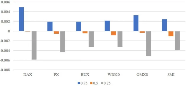
First differences4 were used for all variables and they were tested against unit root by the Im, Pesaran and Shin (2003) test (see Appendix A). The quarterly changes of the stock market volatilities were divided into 25-50-75% quantiles (see Figure 1) to represent
4It provided not just stationary time series but made the interpretation of the results more easier by focusing on the changes of the variables.
the differences among the subsets of the near-to-expected and the mostly extreme values.
This categorisation showed that the German DAX and the Swedish OMXS presented the highest magnitude, while the Hungarian BUX and the Polish WIG20 remained more moderate. These results suggest that there were distinguishable periods of rapidly up- or down swinging volatilities - highlighting the application of quantile regressions.
Figure 1: Quarterly Change of Stock Market Volatility in the 25%, 50% and 75% Quantiles
Source: Authors’ calculation
3.2 Methods
Volatility is time variant as market sentiment changes constantly, so the usage of un- conditional (time-invariant) standard deviation would be misleading. Persistence is an- other important property, since heteroscedasticity represents the presence of high and low volatile periods, which means that if the market was unsure to price in an asset (volatility was high) it would be uncertain tomorrow as well. Such persistence can be captured by different GARCH models, since they can be fitted to estimate conditional (time-variant) standard deviations, following Cappeiello et al. (2006).
GJR GARCH(p,o,q) models can be useful to capture volatility developments, their clustering in time (heteroscedasticity) and their asymmetric occurrence (volatility in- creases if the return is positive or negative). Asymmetric GARCH models can be intro- duced via
( St−i− = 1, if εt−i <0
St−i− = 0, if εt−i ≥0 as a sign asymmetric reaction to decreasing returns.
GJR GARCH (p,o,q) can be written (7):
σt = ω+
p
X
i=1
αi|εt−i|+
o
X
i=1
γiSt−i− |εt−i|+
q
X
j=1
βiσt−j (7)
whereσt2 represents present variance, ω is a constant term, p denotes the lag number of squared past ε2t−i innovations with αi parameters, while q denotes the lag number of past σt−j2 .variances with βi parameters to represent volatility persistence.
Quantile models are based on quantiles of the conditional distribution of the re- sponse variable are expressed as functions of observed covariates. While classical lin- ear regression assumes that grouped data means fall on some linear surface, and the parameters can be estimated on this basis. Least squares regression offers a model:
minµ∈RPn
i=1(yi−µ)2 for randomy andµunconditional population mean. The quantile regression follows a similar approach to conditional quantile functions: the scalar µ is replaced by a parametric function and ξ(xi, β) estimates of the conditional expectation function with a ρτ(.) absolute value function that yields the τth sample quantile as its solution: minβ∈RρPn
i=1ρτ(yi− ξ(xi, β)) (Koenker and Hallock, 2001).
For panel data, according to Lamarche (2010), it is necessary to consider the classical Gaussian random effects model first (8):
y=Xβ+Zα+u (8)
where Z is an ”incidence matrix” of dummy variables, and α and u are independent random vectors. The parameter of primary interestβ can be estimated by two alternative (fixed and random effect) models. Because the error term u is assumed to be mean zero and orthogonal to the independent variables, the conditional mean function of the unob- served effects model is: E(yi,t |xi,t, αi) =x0i,tβ+αi, whereyi,tis the response,xi,tis the vec- tor of covariates, andαiis an individual fixed effect. For quantile panel regression, it is nec- essary to use an analogous conditional quantile model: QYi,t(τj |xi,t, αi) =x0i,tβ(τj) +αi for all quantiles τj in the interval (0, 1). The individual effect is assumed not to represent distributional shift, since it is unrealistic in the case of the small number of individual observations. Therefore, the individual specific effect αi is the pure location shift effect on the conditional quantiles of the response. It is necessary to test the slope equality across quantiles to show that linear models can lead to inadequate conclusions for the specific quantiles, since there is a link between the explanatory and dependent variables.
Therefore, coefficients of the estimated quantiles are valid for cases of p<0.1. There is also a test for symmetry between quantiles to check the heterogeneous impact of the ex- planatory variables, suggesting major discrepancies when comparing the upper and lower tails of the distribution (Skrinjaric, 2018).5
To simplify the interpretation of our results, we have decided to compare only the 25%
and 75% quantiles with the linear panel model. This paper employed random effect (RE) panel regression to backtest the results of the quantile regressions, where the Hausman- test p>0.05 values suggested the usage in all cases.
5We used Eviews 11 econometric software, with the following calibration for the quantile panel regres- sion model: Huber Sandwich Standard Errors & Covariance, Sparsity method: Kernel (Epanechnikov) using residuals, Bandwidth method: Hall-Sheather, bw=0.10052.
4 Results
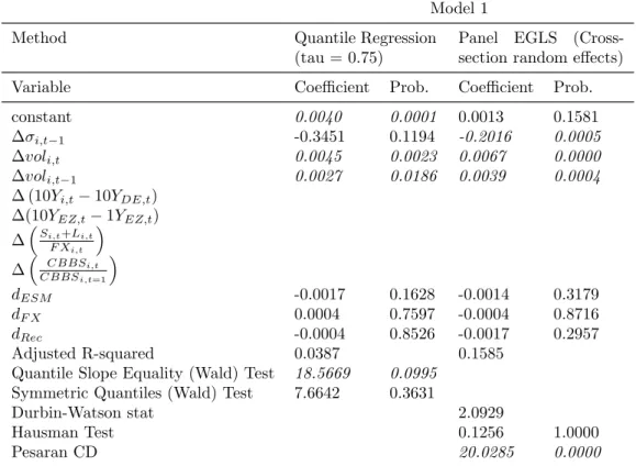
The 25% quantile represents the cases when volatility has a dramatic decrease (market is calming down), while the 75% quantile represents an increasing volatility (market is stressed). All model proved to be functional. Panel RE models had no autocorrelation at the residuals and Hausman-test had appropriate results, but all of them suffered from cross-dependency. Quantile panel regressions had significant quantile slope (so the model has an added value, compared to the RE estimation), but the data remained symmetric.
First, let’s see the variables which were not directly affected by the central bank balance sheet. Stock market index volatility increased when market turnover increased regardless of the fact that we analysed the near-extreme quantiles or the entire sample for all the models - presenting a robust result (see Tables 3 and 4).
Table 3: Results of the Quantile Regression(25%) and the General Panel RE Model
Model 1
Method Quantile Regression
(tau = 0.25)
Panel EGLS (Cross- section random effects)
Variable Coefficient Prob. Coefficient Prob.
constant -0.0034 0.0000 0.0013 0.1581
∆σi,t−1 -0.1966 0.0020 -0.2016 0.0005
∆voli,t 0.0035 0.0042 0.0067 0.0000
∆voli,t−1 0.0016 0.1290 0.0039 0.0004
∆ (10Yi,t−10YDE,t)
∆(10YEZ,t−1YEZ,t)
∆S
i,t+Li,t F Xi,t
∆ CBBS
i,t
CBBSi,t=1
dESM 0.0015 0.1304 -0.0014 0.3179
dF X -0.0001 0.9719 -0.0004 0.8716
dRec -0.0086 0.0055 -0.0017 0.2957
Adjusted R-squared 0.1424 0.1585
Quantile Slope Equality (Wald) Test 18.5669 0.0995 Symmetric Quantiles (Wald) Test 7.6642 0.3631
Durbin-Watson stat 2.0929
Hausman Test 0.1256 1.0000
Pesaran CD 20.0285 0.0000
Note: Significant (p<0.1) values are indicated in italics. Source: Authors’ calculation
For Model 2 (funding conditions), the general RE model suggested that a steeper yield curve and increasing yield premium increases volatility which is parallel with the intu- ition. However, a steeper yield curve in the Eurozone caused a significant decrease in the volatility under the 25% quantile case which is surprising. This calming influence might be interpreted as the restoration of term-premium in the Eurozone which was the benchmark of the recovering market expectations about inflation - what was considered as a good sign during the 2010s close-to-deflation period. Meanwhile, steepness had no significant impact on the market volatility under its dramatic increase (75% quantile) which means
Table 4: Results of the Quantile Regression(75%) and the General Panel RE Model
Model 1
Method Quantile Regression
(tau = 0.75)
Panel EGLS (Cross- section random effects)
Variable Coefficient Prob. Coefficient Prob.
constant 0.0040 0.0001 0.0013 0.1581
∆σi,t−1 -0.3451 0.1194 -0.2016 0.0005
∆voli,t 0.0045 0.0023 0.0067 0.0000
∆voli,t−1 0.0027 0.0186 0.0039 0.0004
∆ (10Yi,t−10YDE,t)
∆(10YEZ,t−1YEZ,t)
∆S
i,t+Li,t
F Xi,t
∆ CBBS
i,t
CBBSi,t=1
dESM -0.0017 0.1628 -0.0014 0.3179
dF X 0.0004 0.7597 -0.0004 0.8716
dRec -0.0004 0.8526 -0.0017 0.2957
Adjusted R-squared 0.0387 0.1585
Quantile Slope Equality (Wald) Test 18.5669 0.0995 Symmetric Quantiles (Wald) Test 7.6642 0.3631
Durbin-Watson stat 2.0929
Hausman Test 0.1256 1.0000
Pesaran CD 20.0285 0.0000
Note: Significant (p<0.1) values are indicated in italics. Source: Authors’ calculation
that valuation was hardly affected by external term premium (see Tables 5 and 6).
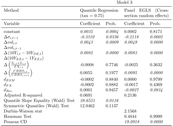
Meanwhile, country-specific yield premiums contributed to the volatility increase not just for the quantiles but for the general set of data for Model 2 and 3. These impressive results indicate the still-existing importance of the interest rate parity. Second, focusing on the central bank balance sheet can help us to identify the possible effects of unconventional monetary instruments. The market maker of last resort function of the central bank is supposed to reinforce domestic funding conditions through the accumulation of domestic public and private bonds, while the lender of last resort function can be captured though increased lending activity (see Tables 7 and 8).
However, the degree of freedom of the sample central banks is not clear, since the majority of the literature focused on the key central banks (which is the ECB for our sample). Naturally, if we focus only on the general RE model (where the adjusted R-square was elevated), the increasing size of the central balance sheet (as a sign of some sort of accumulation of lending, domestic securities or foreign exchange reserves) contributes to an increase in stock market index volatility. However, in the 25% quantile, when volatility was decreasing dramatically (market certainty about valuation recovered), an increased lender- or market maker of last resort activity was able to calm the nerves. On the other hand, this increased (unconventional) activity proved to be insignificant both under near- extreme (75% quantile) volatility increase and the general set of data, making this result less robust.
Table 5: Results of the Quantile Regression(25%) and the General Panel RE Model
Model 2
Method Quantile Regression
(tau = 0.25)
Panel EGLS (Cross- section random effects)
Variable Coefficient Prob. Coefficient Prob.
constant -0.0042 0.0000 0.0007 0.4749
∆σi,t−1 -0.1658 0.0010 -0.2316 0.0001
∆voli,t 0.0033 0.0002 0.0050 0.0000
∆voli,t−1
∆ (10Yi,t−10YDE,t) 0.0034 0.0383 0.0078 0.0002
∆(10YEZ,t−1YEZ,t) -0.0051 0.0001 0.0029 0.1622
∆S
i,t+Li,t F Xi,t
∆ CBBS
i,t
CBBSi,t=1
dESM 0.0017 0.0664 -0.0001 0.9474
dF X 0.0001 0.9321 -0.0003 0.8899
dRec -0.0066 0.0046 -0.0029 0.0849
Adjusted R-squared 0.1650 0.1722
Quantile Slope Equality (Wald) Test 28.4463 0.0124 Symmetric Quantiles (Wald) Test 10.3062 0.2442
Durbin-Watson stat 2.1915
Hausman Test 0.0943 1.0000
Pesaran CD 21.0548 0.0000
Note: Significant (p<0.1) values are indicated in italics. Source: Authors’ calculation
Table 6: Results of the Quantile Regression(75%) and the General Panel RE Model
Model 2
Method Quantile Regression
(tau = 0.75)
Panel EGLS (Cross- section random effects)
Variable Coefficient Prob. Coefficient Prob.
constant 0.0039 0.0001 0.0007 0.4749
∆σi,t−1 -0.3764 0.0092 -0.2316 0.0001
∆voli,t 0.0038 0.0055 0.0050 0.0000
∆voli,t−1
∆ (10Yi,t−10YDE,t) 0.0081 0.0000 0.0078 0.0002
∆(10YEZ,t−1YEZ,t) 0.0024 0.3622 0.0029 0.1622
∆S
i,t+Li,t
F Xi,t
∆ CBBS
i,t
CBBSi,t=1
dESM 0.0000 0.9945 -0.0001 0.9474
dF X -0.0008 0.6133 -0.0003 0.8899
dRec -0.0006 0.6920 -0.0029 0.0849
Adjusted R-squared 0.0634 0.1722
Quantile Slope Equality (Wald) Test 28.4463 0.0124 Symmetric Quantiles (Wald) Test 10.3062 0.2442
Durbin-Watson stat 2.1915
Hausman Test 0.0943 1.0000
Pesaran CD 21.0548 0.0000
Note: Significant (p<0.1) values are indicated in italics. Source: Authors’ calculation
Table 7: Results of the Quantile Regression(25%) and the General Panel RE Model
Model 3
Method Quantile Regression
(tau = 0.25)
Panel EGLS (Cross- section random effects)
Variable Coefficient Prob. Coefficient Prob.
constant -0.0037 0.0000 0.0002 0.8171
∆σi,t−1 -0.1650 0.0134 -0.2118 0.0002
∆voli,t 0.0021 0.0787 0.0049 0.0000
∆voli,t−1
∆ (10Yi,t−10YDE,t) 0.0016 0.6242 0.0083 0.0000
∆(10YEZ,t−1YEZ,t)
∆S
i,t+Li,t F Xi,t
-0.0034 0.0131 -0.0025 0.3632
∆ CBBS
i,t
CBBSi,t=1
0.0023 0.4502 0.0095 0.0000
dESM 0.0014 0.1719 0.0000 0.9799
dF X 0.0002 0.8937 -0.0017 0.4369
dRec -0.0085 0.0053 -0.0027 0.0834
Adjusted R-squared 0.1395 0.2136
Quantile Slope Equality (Wald) Test 28.6551 0.0116 Symmetric Quantiles (Wald) Test 12.9462 0.1137
Durbin-Watson stat 2.1568
Hausman Test 0.4844 0.9999
Pesaran CD 19.0918 0.0000
Note: Significant (p<0.1) values are indicated in italics. Source: Authors’ calculation
Table 8: Results of the Quantile Regression(75%) and the General Panel RE Model
Model 3
Method Quantile Regression
(tau = 0.75)
Panel EGLS (Cross- section random effects)
Variable Coefficient Prob. Coefficient Prob.
constant 0.0035 0.0004 0.0002 0.8171
∆σi,t−1 -0.3310 0.0336 -0.2118 0.0002
∆voli,t 0.0043 0.0009 0.0049 0.0000
∆voli,t−1
∆ (10Yi,t−10YDE,t) 0.0082 0.0000 0.0083 0.0000
∆(10YEZ,t−1YEZ,t)
∆S
i,t+Li,t
F Xi,t
-0.0008 0.7746 -0.0025 0.3632
∆ CBBS
i,t
CBBSi,t=1
0.0055 0.1977 0.0095 0.0000
dESM -0.0002 0.8840 0.0000 0.9799
dF X -0.0002 0.8882 -0.0017 0.4369
dRec 0.0001 0.9457 -0.0027 0.0834
Adjusted R-squared 0.0691 0.2136
Quantile Slope Equality (Wald) Test 28.6551 0.0116 Symmetric Quantiles (Wald) Test 12.9462 0.1137
Durbin-Watson stat 2.1568
Hausman Test 0.4844 0.9999
Pesaran CD 19.0918 0.0000
Note: Significant (p<0.1) values are indicated in italics. Source: Authors’ calculation
5 Conclusion
Regardless of the fact that stock markets are generally not targeted by the monetary policy, they have an important benchmark function in the representation of the asset prices and future cash-flow expectations. Since stock market volatility indicates investors’
certainty about the listed companies’ future cash-flows, the discount rate is influenced by the monetary policy. Unconventional monetary policy became the ”new normal” in the 2010s, and European small and open economies adapted its instruments. However, the efficiency and the nature of the impact has still not been settled in the literature.
Contributing to the solution of this puzzle in the literature, we modelled the changes of the conditional volatility, through the analysis of the domestic and external funding conditions. This paper identified two variables, which supported major decreases in stock market volatility next to the trading volume: the yield premium (as a partially external factor) and the increased domestic lending and security accumulation of the central bank (as a factor of domestic economic policy). Therefore, we can support the claim that unconventional monetary policy can have beneficial calming influence not only on the key central banks, but also on open and relatively small economies.
References
Acs, A. (2014). P´´ enzint´ezeti M´erlegadatok Monet´aris Politikai ´Ujra´ertelmez´ese a Br´ok- erkeresked˝o Szervezetek Re´algazdas´agi ´es Likvidit´asi Jelent˝os´ege. K¨ozgazdas´agi Szemle, 59(2):166–192.
Albertazzi, U., Becker, B., and Boucinha, M. (2018). Portfolio Rebalancing and the Trans- mission of Large-Scale Asset Programmes: Evidence from the Euro Accountingrea. ECB Working Paper No. 2125. Available at SSRN:https://ssrn.com/abstract=3116084.
Belke, A. and Beckmann, J. (2015). Monetary Policy and Stock Prices - Cross-Country Evidence from Cointegrated VAR Models.Journal of Banking and Finance, 54:254–265.
Bernanke, B. S. and Reinhart, V. R. (2004). Conducting Monetary Policy at Very Low Short-Term Interest Rates. American Economic Review, 94(2):85–90.
Blot, C., Creel, J., Hubert, P., Labondance, F., and Ragot, X. (2017). Financial Stability and the ECB. Sciences Po Publications. Info:hdl:2441/35ph3mv7tn8, Sciences Po.
Bohl, M. T., Siklos, P. L., and Sondermann, D. (2008). European Stock Markets and the ECB’s Monetary Policy Surprises. International Finance, 11:117–130.
Borio, C. and Disyatat, P. (2010). Unconventional Monetary Policies: An Appraisal. The Manchester School, 78:53–89.
Buiter, W. and Sibert, A. (2008). The Central Bank as the Market-Maker of Last Resort:
From Lender of Last Resort to Market-Maker of Last Resort.The First Global Financial Crisis of the 21st Century, 171.
Cappeiello, L., Engle, R. F., and Sheppard, K. (2006). Asymmetric Dynamics in the Correlations of Global Equity and Bond Returns. Journal of Financial Econometrics, 4:537–572.
Chatziantoniou, I., Duffy, D., and Filis, G. (2013). Stock Market Response to Monetary and Fiscal Policy Shocks: Multi-Country Evidence. Economic Modelling, 30:754–769.
Chen, Q., Filardo, A., He, D., and Zhu, F. (2016). Financial Crisis, US Unconventional Monetary Policy and International Spillovers. Journal of International Money and Finance, 67:62–81.
Conover, C. M., Jensen, G. R., Johnson, R. R., and Mercer, J. M. (1999). Monetary Envi- ronments and International Stock Returns. Journal of Banking and Finance, 23:1357–
1381.
Czelleng, A. (2019). A Visegr´adi Orsz´agok P´enz¨ugyi Integr´aci´oja: A R´eszv´eny- ´es K¨otv´enypiaci Hozamok, Valamint a Volatilit´as Egy¨uttmozg´as´anak Vizsg´alata Wavelet
´es Kopula Tesztekkel. Statisztikai Szemle, 97(4):347–363.
Damodaran, A. (2011). Little Book of Valuation. John Wiley and Sons.
Dong, F., Miao, J., and Wang, P. (2020). Asset Bubbles and Monetary Policy. Review of Economic Dynamics, 37(1):68–98.
Dooley, M. P. (2014). Can Emerging Economy Central Banks be Market-Makers of Last Resort? BIS Paper, (79).
Eksi, O. and Tas, B. K. O. (2017). Unconventional Monetary Policy and the Stock Market’s Reaction to Federal Reserve Policy Actions. The North American Journal of Economics and Finance, 40:136–147.
Eser, F. and Schwaab, B. (2016). Evaluating the Impact of Unconventional Monetary Policy Measures: Empirical Evidence from the ECB’s Securities Markets Programme.
Journal of Financial Economics, 119(1):147–167.
Falagiarda, M., McQuade, P., and Tirp´ak, M. (2015). Spillovers from the ECB’s Non- standard Monetary Policies on Non-euro Area EU Countries: Evidence from an Event- Study Analysis, No. 1869. ECB working paper.
Farmer, R. E. A. (2013). 2013 John Flemming Memorial Lecture: Qualitative Easing - A New Tool for the Stabilisation of Financial Markets. Bank of England Quarterly Bulletin, 53(4):405–413.
Fausch, J. and Sigonius, M. (2018). The Impact of ECB Monetary Policy Surprises on the German Stock Market. Journal of Macroeconomics, 55:46–63.
Frankel, J. (2011). Monetary Policy in Emerging Markets. In Friedman, B. M. and Woodford, M., editors, Handbook of Monetary Economics, pages 1441–1499. Elsevier.
Fratzscher, M., Duca, M. L., and Straub, R. (2016). ECB Unconventional Monetary Policy: Market Impact and International Spillovers. IMF Economic Review, 64(1):36–
74.
Gal´ı, J. (2013). Monetary Policy and Rational Asset Price Bubbles. Working paper, National Bureau of Economic Research.http://www.nber.org/papers/w18806.
Gal´ı, J. and Gertler, M. (2007). Macroeconomic Modeling for Monetary Policy Evaluation.
Journal of Economic Perspectives, 21:25–45.
Gjerde, Ø. and Sættem, F. (1999). Causal Relations Among Stock Returns and Macroeco- nomic Variables in a Small, Open Economy.Journal of International Financial Markets, Institutions and Money, 9:61–74.
Gray, S. and Talbot, N. (2007). Developing Financial Markets. Bank of England Hand- books in Central Banking, (26).
Gruen, D., Plumb, M., and Stone, A. (2005). How Should Monetary Policy Respond to Asset-Price Bubbles? International Journal of Central Banking, 1(3).
Haincourt, S. (2018). The Nature of the Shock Matters: Some Model-Based Results on the Macroeconomic Effects of Exchange Rate. In Ferrara L., Hernando, I. and Marconi, D., editors, International Macroeconomics in the Wake of the Global Financial Crisis, pages 233–247. Springer.
Haitsma, R., Unalmis, D., and de Haan, J. (2016). The Impact of the ECB’s Conventional and Unconventional Monetary Policies on Stock Markets. Journal of Macroeconomics, 48:101–116.
Heng, Y. K. and Aljunied, S. M. A. (2015). Can Small States Be More than Price Takers in Global Governance? Global Governance, 21(3):435–454.
Hosono, K. and Isobe, S. (2014). The Financial Market Impact of Unconventional Mone- tary Policies in the U.S., the U.K., the Eurozone, and Japan. Discussion papers, ron259.
Policy Research Institute, Ministry of Finance Japan.
Ito, T. (2014). We Are All QE-sians Now. Discussion Paper, (2014-E), 5. Institute for Monetary and Economic Studies, Bank of Japan.
Jensen, G. R. and Johnson, R. R. (1995). Discount Rate Changes and Security Return in the U.S., 1962-1991. Journal of Banking and Finance, 19:79–95.
Joyce, M., Miles, D., Scott, A., and Vayanos, D. (2012). Quantitative Easing and Uncon- ventional Monetary Policy-an Introduction. The Economic Journal, 122(564):271–288.
Kaoru, H. and Shogo, I. (2014). The Financial Market Impact of Unconventional Monetary Policies in the U.S., the U.K., the Eurozone, and Japan. Discussion papers No. 259.
Policy Research Institute, Ministry of Finance Japan.
Kenourgios, D., Drakonaki, E., and Dimitriou, D. (2019). ECB’s Unconventional Mon- etary Policy and Cross-Financial-Market Correlation Dynamics. The North American Journal of Economics and Finance, 50.
Kholodilin, K., Montagnoli, A., Napolitano, O., and Siliverstovs, B. (2009). Assessing the Impact of the ECB’s Monetary Policy on the Stock Markets: A Sectoral View.
Economics Letters, 105(3):211–213.
Koenker, R. and Hallock, K. F. (2001). Quantile Regression. Journal of Economic Per- spectives, 15(4):143–156.
Kurov, A. (2010). Investor Sentiment and the Stock Market’s Reaction to Monetary Policy. Journal of Banking and Finance, 34:139–149.
Lamarche, C. (2010). Robust Penalized Quantile Regression Estimation for Panel Data.
Journal of Econometrics, 157(2):396–408.
Laopodis, N. (2010). Dynamic Linkages Between Monetary Policy and the Stock Market.
Review of Quantitative Finance and Accounting, 35:271–293.
Meggyes, B. and V´aradi, K. (2015). A Likvidit´as ´es a Volatilit´as Napon Bel¨uli Kapcsolata.
K¨oz-gazdas´ag, 10:91–112.
Mishkin, F. S. (2001). The Transmission Mechanism and the Role of Asset Prices in Monetary Policy (No. w8617). National Bureau of Economic Research.
MNB (2017). Modern Jegybanki Gyakorlat. Magyar Nemzeti Bank.
Nagy, B. Z. (2008). T˝ozsdei ´es Ingatlanpiaci ´Arbubor´ekok. K¨ozgazd´asz F´orum, 11(1):5–20.
Nakaso, H. (2013). Financial Crises and Central Banks’ ”Lender of Last Resort” Function.
Remarks, Washington, DC, April, 22.
Pirovano, M. (2012). Monetary Policy and Stock Prices in Small Open Economies: Em- pirical Evidence for the New EU Member States. Economic Systems, 36(3):372–390.