Protozoan prédation in batch and continuous culture

culture

C. R. CURDS* and M. J. BAZINf

* Department of Zoology, British Museum (Natural History), London t Department of Microbiology, Queen Elizabeth College,

University of London

1 Introduction . . . . 1 1 5 2 Theory of microbial prey-predator interactions . . . . . 1 1 7 2.1 Kinetics of prédation . . . . 1 1 8 2.2 Prey-predator dynamics . . . . 1 2 0

3 Practice 142 3.1 Batch culture 143

3.2 Continuous culture . . . . 1 5 3 4 Applied aspects . . . 170

References . . . . 1 7 1

1 Introduction

The behaviour of predatory organisms has long been a topic of con- siderable fascination for artist and scientist alike. The image of strength and invulnerability that predators instil in the mind and their asso- ciation with heroic masculine traits was exemplified in Beowulf, one of the earliest English epic poems, and continues today in the falcons and cougars that are so much a feature of men's toiletry and car advertisements. The role of prédation in natural communities and its effect on natural selection played a major part in Darwin's develop- ment of his theories of evolution as is emphasized by Gause (1934) in

115

his basic text on the relationship between prey and predator populations.

Since Darwin's time the underlying concepts of prédation have been expanded to include political and economic considerations perhaps best seen in the works of Karl Marx who equated capitalists with predators and parasites, contending that societies based on such a system were unstable and would eventually die out.

With the exception of Gause's (1934) work, a decade ago it would have been difficult to find literature concerning the interactions of microorganisms except for purely qualitative descriptions, but now interest is gathering momentum and few microbiology meetings are held without some considerable reference to this topic. Bungay and Bungay (1968) reviewed several types of microbial interactions but we have limited ourselves to one - prédation - and have restricted our terms of reference to protozoan predators only. In our view, of all interactions, prédation is of prime importance since it is one of the major steps in the transfer of energy through a biotic community and is thus a significant component of community metabolism. Further- more, to a large extent prédation controls the numbers of prey present and partly determines the species composition of a community of microbes. Many protozoa are predatory and different species will feed on a great variety of microorganisms - from bacteria and algae to fungi and other protozoa (see Sandon, 1932, still the most complete account of the nonbiochemical aspects of the food of protozoa). In addition, the life-cycles of free-living protozoa are simple when com- pared with those of higher animals and so it is not surprising that protozoa are commonly used as experimental organisms.

Prédation dynamics involve the way in which the populations of at least two species change with respect to time as well as to each other.

In order to specify the nature of these changes, whether for purely descriptive purposes or more formally for proposing an hypothesis, it is necessary to formulate them in mathematical terms. This is not merely for convenience or efficiency but for the precision necessary if the description is to be fully understood or the hypothesis to be tested adequately. For these reasons much of the research that has been undertaken on prey-predator dynamics is of a theoretical nature and has involved the proposition and testing of mathematical models. The advantage of this approach is that the wide range of sophisticated methods available to the mathematician may be brought to bear on generating testable predictions from hypotheses. The manipulations

involved in developing a mathematical model are, perhaps, of greatest importance since they impose on the investigator insights into the system he is studying that would be difficult to gain from a purely qualitative approach to the same problem. The disadvantage of a mathematical approach is that the methods used are often unfamiliar to biologists.

We sincerely hope that the section on theory will not immediately deter the biologist from reading it, since it is to him that we aim our remarks and for this reason have concentrated on the methodology underlying the basic mathematical models that have been proposed to explain prey-predator dynamics rather than attempting to detail the extent to which theoretical aspects of the subject have been developed.

In this paper we present some of our views about the way in which microorganisms have been used to study the relations between prey and predator; these studies have been undertaken to investigate both the behaviour of the microorganisms themselves and the prey- predator situation in general. We do not propose to review all the current literature in this field of study but rather to consider those methods of study we favour, prejudiced as this approach may appear to be.

2 Theory of microbial prey-predator interactions

In order to determine the way in which predatory organisms interact with their prey it is necessary to observe in some way the behaviour of the two populations. Observations alone, however, are unlikely to reveal the nature of the underlying mechanisms of interaction and so, within the framework of the scientific method, guesses or hypotheses are made that offer possible explanations for the observations. In order to either confirm or reject a hypothesis it must be stated in a form that allows testable predictions to be made. For dynamic systems this form appears to be of a mathematical nature and therefore much of the literature on prey-predator dynamics is concerned with mathe- matical hypotheses (or models) and the techniques involved in generat- ing predictions from them.

We begin our discussion of microbial prédation by approaching the subject with a simple hypothesis stated in generalized mathematical terms. We assume that the prey population (H) can grow in the absence of predator (P) but growth of the predator itself is dependent on the

presence of prey. Thus we are limiting our discussion to cases of obligate prédation. We further assume that as the number of predators increases so the rate of decrease in the number of prey organisms increases and finally, that the death rates of prey and predator depend on their respective population densities. The equations for change of the two populations with respect to time can be written as

^ = g1H-d1H-f1P, (1)

^ = -df+ff, (2) where g, d and f are functions, which for the moment we will not

specify, representing the way in which the populations grow and die and the effect of prédation.

2.1 KINETICS OF PREDATION

The functions/, d and g in equations (1) and (2) represent the kinetics of a prey-predator system. We now define these functions in the following manner¹ :

gx = specific growth rate of prey = H/Hforfi = dx = 0, d± = specific death rate of prey = i Z / i / f o r ^ = f± = 0, d2 = specific death rate of predator = PjP ïorf2 = 0, fx = specific rate of prédation = ÊjPïovg1 — dx = 0, f2 = specific growth rate of predator = P/P for d2 = 0.

We define the specific feeding rate, i.e. the effect of prédation on the prey population, a s / i / / P .

The specific growth rate of microbial populations is often regarded as being, within limits, exponential. Application of this assumption to the equation for prey population change implies that gx is a constant which we shall call <xv

The assumption that microorganisms grow in an exponential fashion without limit is unreasonable, of course. T h e effect of population density on specific growth rate is incorporated in the Verhulst-Pearl logistic equation (Gause, 1934) which assumes a linear relationship

1 The dot over the symbol for a variable denotes its derivative with respect to time, e.g.

between specific growth rate and population density. Thus

g1 = a1-y1H, (3)

where ax and γχ are constants.

Introduction of a Verhulst term into the specific growth rate function takes account of the abiotic environment in a nonspecific manner.

If it is assumed that a single nutrient limits the growth of the prey organism a more specific relationship between limiting substrate concentration (S) and specific growth rate, μ, is given by the function suggested by Monod (1942) :

* - ' - ré- < ⁴ >

where μΊΆ is the maximum specific growth rate and K, the saturation constant, is the concentration of limiting nutrient when the specific growth rate = /£m/2. It must be stated at the outset of this discussion that this relationship is an arbitrary one. Attempts have been made to analogize this expression with the Michaelis-Menten equation of enzyme kinetics. However, in the latter case a steady state is assumed to occur between the enzyme, substrate and enzyme-substrate complex and this assumption seems to be valid for enzyme systems. A nutrient- organism complex must also be assumed to be at steady state in order for the analogy to hold for the kinetics of microbial growth. It is clear that in a population of microorganisms that is either growing or dying this will not be true and that this complex will only be independent of time when the population of microorganisms itself is at steady state.

Much of the experimental work that has been carried out on chemostat cultures has been with steady-state situations and it is not surprising that the results obtained are often in agreement with those predicted by the Monod relationship. However, as has been shown by Mateles et al. (1965), the way bacteria grow during transition periods is not predicted by this equation.

The specific death rate in many microbial populations growing under favourable conditions is small and often equated to zero. We will consider cases where this is applicable to the prey population but always assume that the predator dies in the absence of prey. The simplest assumption concerning the way the predator organisms die is that the process is exponential and so for the prey, d± = 0 and for the predator, d2 = a2, a constant. We note that in continuous culture the rate of dilution of the system (Z)) may be regarded as a nonspecific death term.

5 ^AIA

The specific rate of prédation and the specific growth rate of the predator are, of course, closely related functions as the process described by the former results in the latter. It is usually assumed that there is a proportionality constant between these two functions. On a biomass basis this is called a yield coefficient which may be defined by

W=f

IA (5)

which expresses the predator biomass produced per unit of prey biomass. Ifj^ a n d /2 are assumed to be directly proportional to prey density then they become

f1 = /J1Ha.ndf% = ßtH,

where the constants βλ and β2 incorporate the growth yield.

Despite the shortcomings of the Monod relationship it does serve as a useful arbitrary description with which to analyse microbial growth and its application has been extended to describe the specific rate of growth of a microbial predator :

^ = ^λ -ττΉ ^{(6) andso} ^ = w^7ry w

where Àm is the maximum specific growth rate of the predator and L is the saturation constant.

2 . 2 PREY-PREDATOR DYNAMICS

Equations (1) and (2) represent the dynamic relationship between a prey and a predator population in which the kinetic functions are not specified. It is possible to predict in general terms the behaviour of the system in the form presented or by making further assumptions of a nonspecific nature. For example it might be proposed that the specific rate of prédation is a function of the number of predators present, i . e . ^ = ^ ( P ) . In this way all the possible réponses of the model may be predicted regardless of the specific nature of the functions involved.

Analyses of this sort have been performed by Lotka (1923), Rescigno and Richardson (1967), Rescigno (1968), Rescigno and Jones (1972) and Waltman (1964). It is also possible to generalize equations (1) and (2) to multispecies systems and so investigate the dynamics of a total community. Such analyses have been carried out in statistical mechanics terms by Kerner (1957), Leigh (1968) andSamuelson (1971).

Lefever and Nicolis (1971) and Nicolis and Prigogine (1971) employed

the theory of nonequilibrium thermodynamics while Goel et al. (1971) used a variety of mathematical techniques for these analyses. It is beyond the scope of this paper to detail these sophisticated mathematical treatments and we will confine our discussion to relatively simple analysis of deterministic mathematical models containing specified kinetic functions.

TABLE 1

Kinetic functions for dynamic models Prey-

specific Model growth rate

to

Prey- specific death rate

w

Predator- specific death rate

W

Specific rate of prédation

C/i)

Predator- specific growth rate

(/2)

Lotka-Volterra (batch) ax 0 a2 ßxH ß2H

Lotka-Volterra

+ Verhulst term (batch) OLX-XH 0 α2 βχΗ β2Η

Monod saturation μ^β D D XmH XmH

(chemostat) Ks + s W(L + H) L + H

Application of the kinetic functions described in the last section to dynamic models is summarized in Table 1 ; they have been used to describe both batch and continuous systems and for convenience we describe in detail the way the simpler functions have been applied to batch cultures first and then extend the description to continuous systems.

2.2.1 Analysis of prédation dynamics

a. Batch culture Batch culture of microorganisms is experimentally analogous to a closed ecosystem. Organisms are grown in containers and there is no input of matter or energy from the external environment except perhaps for gaseous exchange. The most widely employed theoretical framework for studying prey-predator dynamics is the Lotka-Volterra equations, independently derived by Lotka (1925) and Volterra (1926), which when applied to microorganisms assume the system to be closed and also independent of other abiotic factors.

For two species these equations, in their simplest form, are

^ = α,Η-β,ΗΡ, (8)

5-2

^ = - a2P + ß₂HP, ₍₉₎ from which we see that they are the simplest realization of equations

(1) and (2) where gx = al5 dx = 0, d2 = a2, fx = ßxH a n d /2 = ß2H as indicated in Table 1.

The Lotka-Volterra equations are nonlinear and cannot be solved directly. It is possible to simulate solutions for them by numerical methods or on an analogue computer, as is shown in Fig. 1, but most insight into their behaviour has been gained by mathematical analysis.

In order to gain some understanding of the behaviour of the Lotka-

Time

Fig. 1. Analogue computer plot of Lotka-Volterra equations.

Volterra equations it is instructive to consider how the prey population changes with respect to predator density, i.e. to eliminate the depen- dence of these variables on time. Dividing equation (8) by equation (9) yields

dH_ ( α , - Α Ρ ) # ( 1 0 )

which has the solution

dP (-χ2 + β2Η)Ρ>

ß2H-a2logH = αχ log P-ß±P + c. (11)

Here £, the constant of integration, is dependent on the initial con- ditions, i.e. the sizes o f / / a n d P when t = 0. Equation (11) represents a family of closed curves as is shown in Fig. 2, each one predetermined by this constant. From this simple analysis we can expect quantitatively different responses from a Lotka-Volterra system depending upon the starting conditions.

Inspection of Fig. 2 reveals that the larger curves have distinctly flattened edges but the smaller the curves become, the more closely

Prey density

Fig. 2. Solution of the Lotka- Vol terra equations plotted in phase space.

they resemble ellipses. The centre of the curves is called the equilibrium point and the similarity of the curves to ellipses near the equilibrium point has been used by Pielou (1969) to obtain approximate solutions of the equations so that the behaviour of H and P with respect to time may be predicted. We describe here a slightly different approach used by Leigh (1968) (among others) which can be used as a basis for the study of other models of prédation as well as the Lotka-Volterra equations. In essence we consider the behaviour of the differential equations near the equilibrium point where the values of H and P are small. Because of this characteristic the products of these variables are very small and their effect assumed to be negligible. Elimination of these second-order terms yields a set of differential equations which can be solved analytically.

The equilibrium point of a system is defined such that all the deriva- tives are equal to zero. Application of this definition to equations (8) and (9), i.e. dHjdt = dP/dt = 0, yields

a =ir ^df -% ⁽¹²⁾

where the tilde represents an equilibrium value. Both ß and P will be finite, positive values but if we consider the variables defined by

*! = 7 7 - # a n d x2 = P-P, (13)

then at the equilibrium point these new variables x± = xx and x2 = x2

will both be zero. Substituting for H and P in equation (8) gives

§ = o^+tfj-Äfo + tf) (*, + /») (14)

which, when multiplied out, becomes

—1 = αχχλ + αλΗ—β1χ1χ2 — β^Ρ — βχχ2Η—βλΗΡ.

As we are considering the behaviour of the system near the equilibrium point where x± and x2 have small values, their product, χχχ2, will be very small and so we may neglect the term β1χ1χ2. Furthermore, since from (12)

then equation (14) reduces to

§ = -A^,· (is)

In a similar fashion substitution of the new variables into equation (9) followed by linearization yields

^ = / A (16)

We now differentiate equation (15) to obtain dt^{2 Pl} dt ' After substitution of (16)

^ = -β,ββΡχ,, therefore from (12),

d²x

■^Γ + « ι^αΛ = ° · (^{1 7})

This is the equation of a harmonic oscillator and has well-known properties. The solution of (17) is

xx = A' cos [(θια2)*ί + 0 ] , (18) where A' and φ are constants of integration. Converting back to the

original variables we can obtain Pielou's (1969) equations:

H =ψ + ψΑ cos [(α,α^ί + φ]. (19)

H2 P2

Using similar methods the analogous expression for the predator can be shown to be

P = l + l ^ i l r i n t f o a j t f + fl. (20) On the basis of these results we can state that, near the equilibrium point, the Lotka-Volterra equations predict that both prey and predator populations vary sinusoidally with equal periods,

T = 2ττ/(α1α2)£. In contrast, the amplitudes of the oscillations depend on the integration constant A and thus on the initial conditions; for the prey organism the amplitude is Α<χ2\β2 and for the predator, (Aa^lßj) (oc2locx)i. The other constant of integration, φ, is the phase angle and depends on the value of the variables at zero time. If we let the prey population be at its maximum at this time then φ = 0.

We also see that prey and predator are one quarter T out of phase with each other, with the prey increasing in density first, because prey density is described by a cosine function and predator density by a sine function.

The mean sizes of each population over one period or over many periods is equal to its equilibrium value :

1 C^^+T 1 C^e an

1 Hat = \im±\ Hàt = °^

JU 0-+OO V JO Hz

(21)

1 C^to+T 1 C^e a,

i J Pdt = lim±\ Pdt = %.

In order to obtain a fuller understanding of the Lotka-Volterra equations and other models of prédation it is necessary to understand how linear differential equations are solved. If we set S^x1 = d ^ / d /² and 2xx = d^/d/ then equation (17) may be written as

(^ + c1&+c2)x1 = 0, (22)

where c2 = α±α2 and c± = 0. We now substitute the differential operator {β) by m and eliminate xx to obtain what is called the characteristic equation :

m² + c1m + c2 = 0. (23)

Now the general solution of equation (22) is

xx = axe^m^ + a2e^m^^ti (24)

where ax and a2 are constants. The characteristic exponents, m1 and m g, are obtained by solving the characteristic equation for m using the quadratic formula :

m = Ζ£ΐ±ψ±Α\

)

It is immediately apparent that the nature of m1 and m2 depend on the magnitude and sign of q and whether the expression c\ — \c2 is positive or negative. We will consider the possibilities in turn.

When c\ > 4c2 the characteristic exponents are either both positive, both negative or one is positive and the other negative. If both of the roots are positive the exponential terms in the characteristic equation become larger as time increases and the system in these cases is unstable.

If, on the other hand, the characteristic exponents are both negative then x± will tend towards zero as time tends towards infinity. By definition, from equation (13), H = ft at xx = 0, so the system stabi- lizes at its equilibrium value. When both m1 and m2 have the same sign the equilibrium point generated is called a node. It is stable (Fig. 3) if both are negative and unstable if they are positive. If mx and m2

are of opposite sign, a saddle point results. This is a very apt description of the behaviour of the solution trajectory in phase space as it travels like a marble rolling down from the pommel of a saddle towards the equilibrium point which is at the middle of the saddle. Unless the marble is on a perfectly placed trajectory it will not come to rest at this point, however, but will roll down one of the sides of the saddle.

Thus a saddle point is unstable.

When c\ < 4c2 the term c\ — 4c2in equation (25) becomes negative.

This gives rise to what are called complex conjugate pairs of values for m, i.e.

m = n±pi> (26) where i is defined as the square root of — 1 and n and p depend on the

values of cx and c2. Thus

x1 = αλ exp [(n+pi)t] +a2 exp [(n—pi)t\.

It can be shown (Euler's theorem) that this expression is equivalent to

xi ⁼ [(^öi + ^ß2) cospt+(aj —a2i) sinpt] exp {ni).

If ax and a2 are unequal real numbers then xx has imaginary values,

Equilibrium point

Stable focal point

P i

Stable node

Vortex point (neutrally stable)

P i

Limit cycle

Phase diagram

(©)

|Ô';

Experimental observation ( only predator response shown for clarity )

k

i t

ΛΑΛ ΑΛΛ

H , / Expected

Damped oscillations

Asymptotic approach to .steady state

Undamped oscillations dependent on initial conditions

Undamped oscillations independent of initial conditions

Fig. 3. Possible stable prey-predator interactions.

which is an unrealistic result for the system we wish to represent. For real values of xx we can choose values for ax and a2 such that

a^ — a^i = A' and

αχ + α<ι — Β ' . Then

xx = (Α' sinpt + B' cos pt) exp (nt). (27) Equation (27) has both stable and unstable solutions depending on

the value of n. If n, the real part of the conjugate root, is positive then Λι increases sinusoidally towards infinity as t becomes large and the system is unstable. Such an equilibrium is an unstable focal point.

If n < 0 then the exponential term in equation (27) tends to zero as t tends to infinity. In this case the oscillations of xx become smaller.

As xx = H-H the prey population tends towards its equilibrium value. A similar result can be shown for the predator and the system is thus stable and the equilibrium a stable focal point (Fig. 3).

With n = 0 no damping occurs. This is the case with the transformed Lotka-Volterra variables in equation (17) where the coefficient cx

is the characteristic equation (23) is zero so that equation (25) reduces to

m = ^{± (}~ = ± ( - ' 2 ) * = ±(-«1*2)*·

The solution can therefore be written as

x± = A' sin [(oc1a2)k] +B' cos [{oc1oc2)it],

which is equivalent to equation (18) with A'= J/(aj)i obtained by solving the equation for the initial conditions when it is found that the sine term vanishes.

The phase plane diagram which results from plotting xx against x2

using the linearized Lotka-Volterra equations is similar to the smaller curves in Fig. 2 and is represented in Fig. 3, which summarizes the stable solutions we have discussed. We have seen that the curves for the Lotka-Volterra equations represent a stable system in that per- sistent, undamped oscillations occur. However, if the system is slightly perturbed the trajectory of any particular curve is changed and will not return to the original trajectory as the effect of the perturbation will be equivalent to changing the initial conditions. In this sense then the system is unstable. This sort of stability is called neutral stability and is defined by a characteristic equation which has complex conjugate roots with no real parts. The equilibrium point that it represents is called a vortex point (Fig. 3). It is of interest here to remark on a conclusion of Goel et al. (1971) which predicts that only an even number of species will be able to survive in a Lotka-Volterra system. We can now see how such a prediction arises. We have shown that for a two- species "Lotka-Volterra ecology" both species survive only if the characteristic equation produces complex conjugate roots. For a three-species system the quadratic root of equation (25) becomes a cubic root and three values of m are possible, instead of just two. As complex conjugate roots occur only in pairs it is only possible for two of these values to give rise to them. Thus only two of the three variables are capable of producing a stable result. In a stable situation, then, only two species can survive and the third will die out. Thus it can be seen readily that in any " Lotka-Volterra ecology " with an odd number of species the characteristic equation will not allow a stable solution.

Several modifications of the Lotka-Volterra equations have been proposed. We will discuss one which illustrates the effect of taking into account the abiotic environment by including a Verhulst term in the specific growth rate function of the prey. By doing this equations (1) and (2) become

^-aJI-ßJIP-yJP, (28)

Î j j = -a2P+ß2HP. (29)

The equilibrium values for these equations, i.e. solving for (dHjdt) = (dP/df) = 0, are

ft ^α2

A ßißt Linearization gives rise to

^ + 7 χ # ^ + Α / ν ^ ι = 0, where again, x± = H—£t. The characteristic roots are

-y if f ± ( y 2 f f * - 4 / W ^ ) * m — - 2

For y\ft² ^ 4β1β2ϊ}Ρ the square root is a positive real value; if this value is smaller than γ±Η both m1 and m2 are negative and the result is of the form

x± = ax exp ( — Sjt) + a2 exp ( — S2t),

so as t -> oo, x -> 0 and H -> ß. Similarly as t -> oo, P-> P. Thus both prey and predator densities tend monotonically towards stable steady states because the roots of the characteristic equation are real and negative. In phase space this solution corresponds to the trajectory indicated in Fig. 3 and is a stable node.

When yf/?² < ^βχβ2ϋΡ the characteristic equation has complex conjugate roots and the equilibrium is a focal point. If the real parts of these roots are positive then the solution is unstable. For negative real parts the behaviour of the solution is oscillatory and of the form

x± = Ac exp {-ht) cos (ω^ + φ),

where h = 7 i ^ / 2 and

ωΛ

'Mje-(»g)f-

This equation is the same as that for a linear oscillator with friction.

Strictly speaking the solution is not periodic but the time between successive maxima of xly the conditional period, is constant and equal to 2π/ων The oscillations damp according to the value of A which is called the damping coefficient. The conditional amplitude of the oscillations, Ac, and the phase angle, φ, are functions of the initial conditions of the system.

b. Continuous culture Population dynamics in a continuous culture are controlled by the rate of flow through the system. In chemostat culture, where the system is assumed to be well mixed and the rate of flow (F) into the culture vessel (of volume V) is the same as the rate of output, this flux is governed by the dilution rate, D = F/V. For a single species of density X growth in a chemostat is described simply as

^ = μΧ-ΌΧ, (30) where μ is the specific growth rate of the organism. For a two-species

prey-predator system the dynamics depend on the way in which prey and predator interact. If these interactions are of the type implicitly assumed by the Lotka-Volterra equations the defining equations for prey (H) and predator (P) are

^ = μΗ-DH-frHP, (31)

¥ = -fP-DP+ß^HP. (32) Here i/r is the specific rate of death of the predator. I t can be seen

readily that these equations are analogous to (8) a n d (9) with OL1 = μ — D and a2 = ifr + D. Thus addition of a flow term to the Lotka-Volterra equations does not alter their form and the general solutions will be the same. The stable solution for these equations was found to be a vortex and this will not be changed by altering the experimental parameter, Z), within the limits of a stable result. What will change are the trajectories described in phase space and the values of ft and P which define the equilibrium points. As the trajectories

are also dependent upon the initial conditions repeatable experimental results confirming these predictions would be difficult to obtain.

T h e effect of a Verhulst term added to a Lotka-Volterra open ecosystem is obtained by substituting for ax and a2 in equations (28) and (29) in the same way. In this case the type of stable solution that is obtained depends on αλ and a2 and so will be determined, in part, by the value of D. In general an increase in D will result in more rapid damping of the oscillations and eventually the disappearance of all oscillations. At low dilution rates, then, we might expect a stable focal point (Fig. 3) while at higher dilution rates a stable focus is generated.

Using Monod kinetics for prey and predator growth in a chemostat yields the following equations for populations change:

at " K + S W(L + H) ^{ôô)

d P λ^ΗΡ

at L + H ^r- ^[OV

Here W is the stoichiometric coefficient or yield of predator per unit of prey and is assumed to be constant. I n contrast to the Lotka- Volterra equations with a Verhulst term, employing the Monod function allows us to specify the behaviour of the abiotic environment represented by the concentration of limiting nutrient:

— = D(S0-S)-Y(£ + s y (35)

where S0 is the concentration of nutrient in the input medium and Y is the yield constant for the prey organism.

These equations may be linearized near equilibrium a n d the trajectories of the solutions traced in three-dimensional (prey, predator and substrate) phase space. This analysis has been published in detail by Canale (1969, 1970) and will not be repeated here. The linearized equations admit to three equilibrium points defined by

jff=p = 0; S = S0 (a)

P = 0; 3+Î}/Y = S0 (b) (36)

Ë P

γ + ψϊγ+8 = ^So (^c)

The only equilibrium in which both prey and predator survive, and thus the only one of interest in the present context, is 36 (c). Equilibrium

16 (c) has three stable solutions depending on the dilution rate of the system. At comparatively high dilution rates such that neither species washes out, both prey and predator populations change monotonically towards steady-state values and a stable node (Fig. 3) is generated.

At lower dilution rates a stable focal point (Fig. 3) is generated and the populations exhibit damped oscillations. At even lower dilution rates the system gives rise to sustained oscillations in all three variables.

In phase space the trajectories are closed curves. Effectively what is happening is that the characteristic equation gives rise to an unstable focal point but the solution trajectory is bounded so that the variables cannot exceed values imposed by the parameters of the system. This type of solution is called a limit cycle (Fig. 3) and is different from the vortex point of the Lotka-Volterra equations in that the cycles are independent of the initial conditions and after small perturbations the solution trajectory will return to its original path. A system which gives rise to limit cycles may thus be regarded as strictly stable (i.e.

according to the definition of Liapounof (Andronov et al.y 1966)).

Limit cycles cannot be found directly by analysing the linearized equations as they are a result of second-order terms.

Several modifications of the Monod (1942) term have been proposed (Contois, 1959; Kono and Asai, 1969; Topiwala, 1971; Yano and Koga, 1973) and recently Jost et al. (1973b) have proposed what they call a multiple saturation model to represent the specific rate of growth of a predatory microorganism in chemostat culture. This expression takes the form

λ ΡΗ^η

i = l

The growth of the predator is assumed to take place in n stages, each stage with an effective saturation constant of L{. For n = 1 the expres- sion reduces to the Monod term. The authors derive this expression by assuming that "pseudo-steady states" of the hypothetical prey-predator complexes occur for each of the n stages of predator growth in the same way that has been suggested for the proposed nutrient-biomass complex by analogy to enzyme kinetics. As has been pointed out, however, it is unlikely that such complexes do remain independent of time in changing systems and this is particularly inappropriate for describing prey-predator dynamics due to the oscillatory responses observed.

The point of studying mathematical models is to gain some insight into the possible mechanisms underlying a given system. The prey- predator models we have discussed so far show that qualitatively different types of response may exist and provide a great deal of theoretical information about the possible behaviour of microbial populations. What these models have not done, and what is needed, is to relate the population dynamics of the system to the way in which the individual prey and predator organisms behave although at least an attempt has been made with the saturation models. There are two ways in which this problem may be attacked ; either individual prey and predator organisms may be studied to determine their mode of inter- action or the population behaviour may be analysed and the behaviour of the individuals inferred from the results. It is the latter method for which chemostat culture is most useful. To date there appears to be no satisfactory theory which does relate cellular behaviour to the behaviour of a population even for single-species systems. Ramkrishna et al. (1967) have proposed what they call structured models which take explicit account of the physiological state of the microorganisms, and Fredrickson et ai (1970) put forward convincing arguments in support of such an approach. In effect they say that the physiological state and therefore the rate of reaction of a cell changes as a function of its age and that representing a population of cells by a single time-dependent variable is insufficient; the population is composed of cells in different states and each state should be represented on a population basis. A specific example of a structured model is that proposed by Williams (1967) for a single species growing in either batch or continuous culture.

Merely by regarding a cell as being divided into a structural-genetic and a synthetic portion several fundamental observations of growth dynamics are predicted, including the distinction between change in biomass and number densities. The chief argument against employing models of this type for multispecies systems is that too much complexity is involved in the final mathematical formulations. Although it is quite possible to produce sets of models for such systems based on the approach of Williams (1967), the resulting equations contain a great many coefficients whose values are unknown and variables which would be difficult, if not impossible, to measure. In general, increasing the number of parameters in a mathematical expression will increase the variety of responses that can be expected. Models of this sort then would be very difficult to test and most probably at this stage in such

investigations represent little more than exercises in curve fitting.

O n the other hand it might be possible to apply analyses of the form proposed by Prigogine and his co-workers (Prigogine and Nicolis, 1971) which specifically relate to the behaviour of nonlinear systems operating far away from equilibrium. Another possible line of approach lies in the new field of mathematics originated by René Thorn which appears to provide a mathematical way of studying the occurrence of sudden changes in systems. This "catastrophe theory" has been applied to morphogenetic events (Thorn, 1970) and its extension into other biological phenomena is to be expected.

2.2.2 Simulation techniques

In order to test any particular dynamic model it is necessary to compare experimental data to the behaviour of the time-dependent variables of the theory. As many biological models are nonlinear and cannot be solved directly by analytical methods it is therefore necessary to gener- ate reliable estimates of these values by some other means. Two methods are commonly employed for accomplishing this : the system of differen- tial equations may be represented by an electrical circuit and solved on an analogue computer or the solutions may be approximated, to any degree of accuracy required, by numerical integration. These methods have the advantage over the linearization technique described in the last section in that the effects of nonlinear terms are taken into account and transient responses to perturbations can be determined with precision.

Details of analogue computer methodology applied to ecological systems are given by Patten (1971) ; the solution of the Lotka-Volterra equations illustrated in Fig. 1 was obtained by this technique and Bungay (1968) and Williams (1967), among others, have used this method for investigating microbial population behaviour. The main advantage of the analogue computer is that it brings the operator into the closest possible contact with the equations under analysis and results can be obtained instantaneously whereas most digital systems do not afford this facility. For this reason small analogue computers are valuable teaching aids but as the magnitude of the parameters in any particular set of equations is restricted by the voltage output of the machine, in many cases the equations must be scaled in order to be analysed by this method. Scaling can be a very complicated

process and it is mainly for this reason that most workers now tend to use numerical techniques in conjunction with a digital computer.

Numerical approximation of the solution of differential equations is accomplished by repeatedly calculating the integrals after very short time intervals, the size of which is called the step size. The smaller the step size, the more accurate are the results. Because step sizes are comparatively small and because for each step considerable arithmetic is involved the only practical way of solving equations in this way is by using a digital computer.

Numerical integration techniques have been considerably simplified by the introduction of purpose-built simulation languages which provide all the facilities of an analogue computer without the restrict- ions imposed by scaling. Such languages have several advantages for biologists with limited mathematical background: firstly, they are simple to learn so that the ecologist can concentrate on the problem at hand rather than details of programming; secondly, the transient behaviour of a model can be examined without recourse to detailed mathematical analysis. Furthermore, for a system whose parameters are known the output from such simulation can be used as a basis for designing experiments and also for fitting the results to those predicted by the model being tested.

Several simulation languages exist but the one most widely used in studies of microbial population dynamics is CSMP (Continuous System Modelling Program) designed for use on IBM 360 series computers.

Instructions for using CSMP are described in the S/360 Users' Manual IBM 20-0367-2 and also by Patten (1971) who emphasizes its applica- tion to ecological models. For convenience we reproduce in Table 2 a CSMP program which represents the interaction between bacterial prey and a protozoan predator under conditions of continuous culture, assuming growth of both organisms to obey Monod kinetics, i.e. the solutions to equations (32), (33) and (34) are simulated. The program may be divided into three parts :

a. Data statements These assign numerical values to constants and parameters as shown in Table 2. As it is not possible to keypunch subscripts or lower case letters the symbols employed are necessarily different from those used in equations (32), (33) and (34) and the following equalities hold: SO = S0, D = Z>, MUMB = /im, KS = K,

TABLE 2

A prey-predator computer program written in the simulation language CSMP/360. (After Curds, 1971a.)

****CONTINUOUS SYSTEM MODELLING PROGRAM****

***PROBLEM INPUT STATEMENTS***

PARAM SR = 2000, D = 0-1, MUMB = 0-6, KS = 4-0, Y = 045 PARAM MUMC = 043, KB = 120, YG = 0-54

INCON SA = 1-96, BA = 90, GA = 45-01 DYNAM

MUB = MUMB*S/(KS + S) MUG = MUMC*B/(KB + B) SDOT = D*SR-D*S-MUB*B/Y BDOT = MUB*B-D*B-MUC*C/YC CDOT = MUG*C-D*G

S = INTGRL (SA, SDOT) B = INTGRL (BA, BDOT) G = INTGRL (CA, CDOT)

TIMER DELT = 001, FINTIM = 2400, PRDEL = 10, OUTDEL = 10 PRINT S, B, C, MUB, MUC

PRTPLT S. B, G

TITLE DYNAMIC MODEL PREDATOR-PREY LABEL DYNAMIC MODEL PREDATOR-PREY END

STOP ENDJOB

YB = Y, MUMC = Xm, KB = L, YC = W. In order to obtain numerical results from differential equations the initial conditions must be specified; these are the concentrations of prey, predator, and limiting nutrient at zero time. They are symbolized by BA, CA and SA respectively.

b. Structural statements These describe the functional relationship (DYNAM) between the variables of the model and so define the system to be simulated. The bacterial population is symbolized by B, the predator by C and the nutrient concentration by S. Statements are written in standard F O R T R A N . The first two statements calculate the specific growth rates of the prey and the predator and the next three statements define new variables SDOT, BDOT and CDOT. The last three statements contain the CSMP function I N T G R L which integrates these variables using initial conditions defined by data statements.

c. Control statements These specify the options relating to the trans- lation and execution of the program. They include the length of time over which integration is required (FINTIM), the step size, which in this program is fixed (DELT) but under CSMP need not be, and allow the numerical values of the variables to be printed (PRINT) and/or plotted (PRTPLT) at specified intervals (PRDEL and OUTDEL, respectively). Other options are available for which the Users' Manual should be consulted.

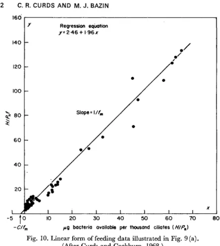
The values of the parameters assigned in Table 2 are those deter- mined experimentally by Curds and Cockburn (1971) for the bacterium Klebsiella aerogenes and the ciliate Tetrahymena pyriformis. Typical results of the simulation are given in Fig. 4. All five variables (bacteria,

0 50 100 150 200 250 300 Time (h)

Fig. 4. Limit-cycle oscillations of populations and their specific growth rates given by the computer program in Table 2. (After Curds, 1971a.)

substrate and ciliate concentrations and the specific growth rates of the two organisms) oscillate in a regular fashion without damping. The stability of the system can be tested by using the analytically calculated equilibrium values as the initial conditions. Even when high precision is used the system begins to oscillate immediately (Curds, 1971a), the amplitude increasing and the wavelength decreasing until stable limit- cycle oscillations are established. Thus even minor perturbation from the equilibrium position generated within the computer results in move- ment away from the equilibrium point towards regular periodic motion.

2 Ö 0 l ·

150

f 100

5 0

200 0

150

1 100

50 (a)

Bacteria

Nutrient t Γ (b)

Nutrient

H «0 20 S

0 1 0 2 0-3 0-4

Dilution rate (h~')

Fig. 5. Effect of dilution rate upon theoretical steady-state values of limiting nutrient and bacteria (a) in the absence of a predator and (b) when a predatory ciliated proto- zoan is present. (Adapted from Curds, 1971a.)

The relationship between dilution rate and the population variables for a single-species chemostat culture is shown in Fig. 5 (a). In compari- son the values obtained when a predator is present, assuming steady states are achieved, are shown in Fig. 5 (b). It can be seen that when a predator is present the steady-state concentration of substrate decreases as the dilution rate is increased whereas the prey and predator popula- tions increase. This is contrary to the situation when a single organism is present. At dilution rates in excess of the critical rate for the ciliate the culture becomes a single species continuous culture and the curves are identical.

The types of equilibria derived analytically may be demonstrated by simulation ; for the kinetic constants used in Table 2 dilution rates from 0-02 to 0-33 h^{_ 1} produce stable limit-cycle oscillations; at D = 0-34 and 0-55 h^{_ 1} damped oscillations occur indicating a stable focal-point solution; at D = 0-36 h^{- 1} a stable node results as the concentrations of bacteria, ciliate and substrate tend to steady-state values monotonically.

At dilution rates above 0-37 h^{_ 1} the ciliate population washes out and (see equation (45)) the bacteria asymptote to steady-state levels (stable node).

Under limit-cycle conditions the frequency of the oscillations depends upon the dilution rate in the way illustrated in Fig. 6. At low dilution rates the frequency is low and increases to a maximum after which it decreases to zero, i.e. steady state is obtained.

The magnitude of the maximum specific growth rate of the predator has a significant effect upon oscillation frequency. High values produce oscillations with low frequencies and as the maximum specific growth rate decreases so the frequency increases. The value of the saturation constant of the ciliate affects both the oscillation frequency and the extreme limits of the oscillating population. Frequency increases with the saturation constant. At high values of the saturation constant the maximum population densities obtained are reduced while the mini- mum population sizes are not so small. Small saturation constants produce the reverse effect.

The effect of varying other parameters can be estimated by varying them one at a time and simulating the results. Increasing the maximum specific growth rate of the prey gives rise to an increase in the frequency of the oscillations ; the saturation constant of the prey has little effect on the periodicity of the system but it does affect the maximum concen- tration of ciliates that can be obtained. The value of K also determines

0-4

— 0·3 l·

ϋ!0·2

0·Ι h

0-2 Dilution rate (h^-1)

0-4

Fig. 6. Effect of dilution rate upon the oscillation frequency of a prey-predator system in a chemostat. (After Curds, 1971a.)

the rate of change in substrate concentration ; at low values the decline in substrate becomes very rapid and simulation often allocates negative values to substrate concentrations in such cases. This, of course, is theoretically and physically impossible and the explanation of the result lies in the mechanics of the numerical technique employed in the simulation language. Several numerical integration methods are available but all of them depend on the step size over which each approximation is performed. For functions which change rapidly such as the case indicated here, the step size must be very small otherwise the result estimated will be inaccurate and the magnitude of the innacuracy may increase as integration proceeds. For the particular example of substrate concentration at low K values the rapid decrease in S results in the calculation of a negative value for this variable as S -> 0 which the integration routine cannot rectify. In this case the error is obvious but inaccurate results, both qualitative and quantitative, may arise which are not so easily noticed. It is therefore wise to include some sort of error analysis when simulation techniques are employed.

Probably the simplest check, but not the most rigorous nor the most efficient, is to run some programs twice using different step sizes to determine if the results differ significantly.

The simulation technique of analysing population dynamics is valuable for studying multispecies systems and for testing specific kinetic functions. Bungay and Paynter (1971) used computer simulation methods to investigate the dynamic behaviour of multicomponent models and included first-order time delays between substrate changes and the response of the growth rate of the microorganisms. These authors argue that when the limiting nutrient concentration is suddenly increased the cells cannot immediately establish the specific growth rate predicted by the Monod function and there is a lag period during which the cellular machinery necessary for the adaptation is produced. On the other hand they state that the growth rate can decline rapidly with no apparent lag if nutrient concentration is decreased. Young, Bruley and Bungay (1970), working with the yeast, Saccharomyces cerevesiae, tested several mathematical ways of representing a delay mechanism and found that a first-order lag fitted their data reasonably well. For these reasons Bungay and Paynter (1971) used unmodified Monod functions when substrate concentrations were declining and the same functions with first-order time lags when substrate concentrations increased. They report that such a time delay caused the substrate concentration to oscillate with much greater amplitude and in par- ticular caused the simulated nutrient concentration to drop to low values. It should be noted, however, that a smaller saturation constant could also give the same result.

The work of Bungay and Paynter (1971) on complex microbial systems also included the effect of a predator feeding on two competing prey organisms. Curds (1974) also tested a number of complex microbial food chains using slightly different kinetic functions. Bungay and Paynter (1971) infer, and Curds (1974) states that the magni- tude of the kinetic constants have a more significant effect on the dynamics of the populations than the detailed form of the kinetic functions.

As computer simulations of microbial interactions are so much simpler to perform than the appropriate laboratory experiments no doubt this theoretical approach will be increasingly employed by microbial ecologists, perhaps at the expense of experimental investi- gation. The danger, already becoming apparent, is that a host of models

will be simulated and appear in the literature. As there are an infinite number of theoretical models such a process is without limit unless it is clearly recognized that solving a set of differential equations will not add to our understanding of ecological processes unless the equations themselves are based on ecological observations. If the introduction of simulation languages does not increase the number of experiments performed on ecological systems, or, even worse, switches the attention of ecologists from observational or experimental approaches to purely theoretical ones, they will have hindered rather than enhanced the progress of ecological research. We believe that theoretical and experi- mental approaches should be integrated ; construction of a mathematical model imposes upon the investigator the responsibility of rigorously defining his assumptions and allows explicit predictions to be made.

Experiment is needed to determine how close these predictions, and thus the assumptions on which they are based, mirror reality. At present our models are incomplete and usually only agree in a qualita- tive manner with results from laboratory cultures. They are even less accurate in describing natural communities of microorganisms. The role of computer simulation as a means of testing dynamic hypotheses and comparing experimental results with theoretical predictions, is rapidly becoming an indispensable technique and in the future will also become of increasing importance in forecasting the behaviour of eco- systems both in the laboratory and in nature.

3 Practice

There are two basic methods of experimentally investigating prey- predator relationships; the first is to use the batch-culture method in which the populations of organisms are isolated from the external environment, and the second is to use the continuous-culture tech- nique in which explicit account is taken of input and output of energy and matter. In the latter method stable conditions such as steady states or sustained oscillations may occur which are of consider- able advantage, as experiments may be run over extended periods of time.

3.1 BATCH CULTURE

Until the introduction of the continuous-culture technique by Monod (1950) all work on the growth kinetics, physiology and bio- chemistry of microorganisms was based on batch-culture methods.

Continuous cultures have not replaced batch methods since the latter have several advantages over the former. The batch-culture method is a comparatively quick and easy way of obtaining reasonable estimates of kinetic data and yield coefficients without major apparatus; indeed batch studies usually precede continuous-culture work. It is possible to work with low population densities and to make the environment spatially heterogeneous, both of which are inapplicable in continuous culture. However, there are also several major disadvantages inherent in batch cultures which can be overcome by the use of continuous- culture techniques. At the onset of batch cultures, the nutrient is usually in excess and there are few organisms, but as the latter grow the nutrient diminishes ; at the same time, the physicochemical properties of the environment change and there will be an accumulation of potentially harmful metabolic products. In spite of the disadvantages, batch culture will continue to play a vital role in prey-predator research and the following account will serve to illustrate its use and adaptability.

3.1.1 Qualitative experimental work

a. Food preferences of protozoa Several authors have reported upon the use of batch cultures in their experiments concerned with the food preferences of protozoa. Many of these workers (Burbanck, 1942;

Curds and Vandyke, 1966; Groscop and Brent, 1964, and others) have used bacteria as the prey and these have been presented, either as suspensions or as streaks on agar plates, to protozoa as their sole food source. This type of work has clearly demonstrated that not all bacteria, in isolation, are suitable for the prolonged survival of all protozoa.

For example, Curds and Vandyke (1966) presented five species of ciliate separately with an excess supply of nineteen strains of different bacteria as the sole food source and they were able to divide the prey into three major categories - toxic, unfavourable and favourable - according to their effect upon the predators.

Apparently certain bacteria, particularly pigmented varieties, are toxic to various protozoa (Chatton and Chatton, 1927; Kidder and

Stuart, 1939; Singh, 1942, 1945, 1946; Brent, 1948; Groscop, 1963;

Groscop and Brent, 1964; Curds and Vandyke, 1966) and the evidence available suggests that the bacterial pigment is frequently the toxic agent. It should be remembered, however, that these data have been obtained from laboratory studies and the significance of these obser- vations when applied to the natural environment remains to be defined.

According to Curds and Vandyke (1966) some bacteria - unfavourable ones - although nontoxic will not support the growth of protozoa indefinitely, whilst others - favourable ones - will do so. In addition, a bacterial strain may be favourable to one protozoon but unfavourable to another. Even within a group of favourable bacteria there is a degree of favourability for a given protozoan species since it has been demon- strated (Curds and Vandyke, 1966) that an excess of different favour- able bacteria will support different maximum growth rates of ciliated protozoa. Perhaps this is not surprising as it is analogous to the situation in osmotrophic microorganisms where the growth rate is dependent upon the identity of the nutrient supplied. Burbanck and Gilpin (1946) even suggested that the measurement of the growth rate of the ciliate Colpidium colpoda could be used as a method for the identification of some

medically important intestinal bacteria.

Although most work of this nature has considered bacteria as the prey organisms some information is available on the feeding activities of amoebae on soil fungi. Heal (1963) presented four species of amoebae with 35 species of fungi; all of the 19 species of yeast were eaten to varying extents and it was suggested that yeasts are a possible food source for soil amoebae. Although the sporangiospores of the 16 fungal species presented were ingested, only those of Paecilomyces elegans and Polyscytalum fecundissimum were actually digested and supported the growth of the amoebae.

b. Food selection Data from batch experimental work imply that protozoa are able to select the organisms to be ingested (Singh, 1942).

For example, Schaeffer (1910) recorded that the ciliate Stentor coeruleus ingested 12 of the 15 Phacus sp. cells supplied while all 13 of the sulphur particles introduced were rejected. Furthermore, S. coeruleus apparently was able to discriminate between two species of Phacus, predominantly accepting P. triqueter and rejecting P. longicaudus. However, no data were given on whether either of the two algal species were actually digested and it is well known that ciliates will ingest apparently useless

particles such as carmine. Many carnivorous protozoa will feed upon certain prey protozoa to the exclusion of others; for example the ciliate Didinium nasutum feeds exclusively upon the ciliate Paramecium caudatum and there are many other well-documented examples (Sandon, 1932). More evidence on food selection has been furnished by Lee et al.

(1966) who used tracer-labelled organisms as a method of studying prey-predator relationships among the foraminifera. They presented more than 50 ³²P or ¹⁴C-labelled axenic species of protists to ten species of foraminifera and found that although all these organisms occur in the natural habitat, the foraminifera selected only certain organisms for ingestion. They found that the yeasts, cyanophytes, dinoflagellates, chrysophytes and most of the bacteria tested were not eaten whereas certain species of diatom, chlorophytes and bacteria were eaten in large quantities. Later, Müller and Lee (1969) found that the identifi- cation of potential food organisms by these methods did not necessarily indicate whether or not they would support the growth of the foramini- fera. These two authors reported their failure to establish bacteria-free cultures of the four foraminifera species supplied with one or two species of algae and observed that in addition bacteria were required for the prolonged survival of the protozoa. This type of work indicates that ingestion of prey is of little significance unless it is accompanied by data on the growth-supporting potentials of the prey.

Almost all the experimental work on the selective abilities of protozoa has been aimed at demonstrating their abilities rather than the quan- titative aspects of the problem and there is clearly an urgent need for work of this nature.

3.1.2 Quantitative experimental work

a. Zoological methods Salt (1967) used a purely zoological approach when he carried out a series of batch experiments on the predatory ciliate Woodruffia metabolica. He found that this ciliate would feed upon three species of the genus Paramecium but not upon bacteria, algae and some other ciliates tested. Salt's (1967) novel method was to introduce washed animals into 0-1 -ml drops of inorganic salts medium under paraffin oil. The oil prevented evaporation yet allowed gaseous exchange and the introduction and removal of organisms during an experiment.

A ciné camera was set to photograph the complete drop at 50-minute intervals so that animals could be counted from the photographic