Nonparametric Statistics

(1)

Nonparametric Statistics

László Györfi

February 3, 2014

(2)

(3)

Chapter 1 Introduction

In this chapter we introduce the problem of regression function estimation and describe important properties of regression estimates. Furthermore, provide an overview of various approaches to nonparametric regression estimates.

1.1 Why to Estimate a Regression Function?

In regression analysis one considers a random vector (X, Y), where X is R^d-valued and Y is R-valued, and one is interested how the value of the so-called response variable Y depends on the value of the observation vectorX. This means that one wants to find a (measurable) functionf :R^d →R, such thatf(X) is a “good approximation ofY,” that is, f(X) should be close to Y in some sense, which is equivalent to making |f(X)−Y|

“small.” Since X and Y are random vectors, |f(X)−Y| is random as well, therefore it is not clear what “small|f(X)−Y|” means. We can resolve this problem by introducing the so-calledL₂ risk or mean squared error of f,

E|f(X)−Y|², and requiring it to be as small as possible.

There are two reasons for considering the L₂ risk. First, as we will see in the sequel, this simplifies the mathematical treatment of the whole problem. For example, as is shown below, the function which minimizes theL₂risk can be derived explicitly. Second, and more important, trying to minimize the L₂ risk leads naturally to estimates which can be computed rapidly.

So we are interested in a (measurable) function m^∗ :R^d →Rsuch that E|m^∗(X)−Y|² = min

f:R^d→RE|f(X)−Y|².

(6)

Such a function can be obtained explicitly as follows. Let m(x) =E{Y|X =x}

be the regression function. We will show that the regression function minimizes the L₂ risk. Indeed, for an arbitrary f :R^d →R, one has

E|f(X)−Y|² = E|f(X)−m(X) +m(X)−Y|²

= E|f(X)−m(X)|²+E|m(X)−Y|², where we have used

E{(f(X)−m(X))(m(X)−Y)}

=E E

(f(X)−m(X))(m(X)−Y) X

=E{(f(X)−m(X))E{m(X)−Y|X}}

=E{(f(X)−m(X))(m(X)−m(X))}

= 0.

Hence,

E|f(X)−Y|² = Z

R^d

|f(x)−m(x)|²µ(dx) +E|m(X)−Y|², (1.1) where µ denotes the distribution of X. The first term is called the L₂ error of f. It is always nonnegative and is zero if f(x) = m(x). Therefore, m^∗(x) = m(x), i.e., the optimal approximation (with respect to theL₂ risk) of Y by a function of X is given by m(X).

In applications the distribution of (X, Y)(and hence also the regression function) is usually unknown. Therefore it is impossible to predict Y using m(X). But it is often possible to observe data according to the distribution of (X, Y) and to estimate the regression function from these data.

To be more precise, denote by (X, Y), (X₁, Y₁), (X₂, Y₂), . . . independent and iden- tically distributed (i.i.d.) random variables with EY² < ∞. Let D_n be the set of data defined by

D_n ={(X₁, Y₁), . . . ,(X_n, Y_n)}.

In the regression function estimation problem one wants to use the data D_n in order to construct an estimate m_n : R^d → R of the regression function m. Here m_n(x) = m_n(x, D_n) is a measurable function of x and the data. For simplicity, we will suppress D_n in the notation and write m_n(x) instead ofm_n(x, D_n).

(7)

In general, estimates will not be equal to the regression function. To compare dif- ferent estimates, we need an error criterion which measures the difference between the regression function and an arbitrary estimate m_n. One of the key points we would like to make is that the motivation for introducing the regression function leads naturally to an L₂ error criterion for measuring the performance of the regression function estimate. Recall that the main goal was to find a function f such that the L₂ risk E|f(X)−Y|² is small. The minimal value of this L₂ risk is E|m(X)−Y|², and it is achieved by the regression functionm. Similarly to (1.1), one can show that theL₂ risk E{|m_n(X)−Y|²|D_n} of an estimate m_n satisfies

E

|m_n(X)−Y|²|D_n = Z

R^d

|m_n(x)−m(x)|²µ(dx) +E|m(X)−Y|². (1.2) Thus the L₂ risk of an estimate m_n is close to the optimal value if and only if the L₂ error

km_n−mk² = Z

R^d

|m_n(x)−m(x)|²µ(dx) (1.3) is close to zero. Therefore we will use theL₂ error (1.3) in order to measure the quality of an estimate and we will study estimates for which thisL₂ error is small.

The classical approach for estimating a regression function is the so-called parametric regression estimation. Here one assumes that the structure of the regression function is known and depends only on finitely many parameters, and one uses the data to estimate the (unknown) values of these parameters.

The linear regression estimate is an example of such an estimate. In linear regression one assumes that the regression function is a linear combination of the components of x= (x⁽¹⁾, . . . , x^(d))^T, i.e.,

m(x⁽¹⁾, . . . , x^(d)) = a₀+

d

X

i=1

a_ix⁽ⁱ⁾ ((x⁽¹⁾, . . . , x^(d))^T ∈R^d)

for some unknown a₀, . . . , a_d ∈ R. Then one uses the data to estimate these parameters, e.g., by applying the principle of least squares, where one chooses the coefficients a₀, . . . , a_d of the linear function such that it best fits the given data:

(ˆa₀, . . . ,ˆa_d) = arg min

a0,...,ad∈R^d





 1 n

n

X

j=1

Y_j−a₀ −

d

X

i=1

a_iX_j⁽ⁱ⁾

2



 .

(8)

- 6

−1 −0.5 0.5 1

0.5

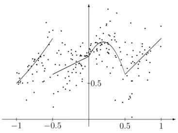
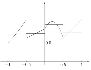
Figure 1.1: Simulated data points.

HereX_j⁽ⁱ⁾ denotes theith component ofX_j and z= arg min_x∈Df(x)is the abbreviation for z∈Dand f(z) = min_x∈Df(x). Finally one defines the estimate by

ˆ

m_n(x) = ˆa₀+

d

X

i=1

ˆ a_ix⁽ⁱ⁾.

Parametric estimates usually depend only on a few parameters, therefore they are suit- able even for small sample sizes n, if the parametric model is appropriately chosen.

Furthermore, they are often easy to interpret. For instance in a linear model (when m(x) is a linear function) the absolute value of the coefficient ˆai indicates how much influence the ith component ofXhas on the value of Y, and the sign of ˆa_i describes the nature of this influence (increasing or decreasing the value of Y).

However, parametric estimates have a big drawback. Regardless of the data, a parametric estimate cannot approximate the regression function better than the best function which has the assumed parametric structure. For example, a linear regression estimate will produce a large error for every sample size if the true underlying regression function is not linear and cannot be well approximated by linear functions.

For univariate X = X one can often use a plot of the data to choose a proper parametric estimate. But this is not always possible, as we now illustrate using simulated data. These data will be used throughout the book. They consist ofn = 200points such that X is standard normal restricted to [−1,1], i.e., the density of X is proportional to the standard normal density on [−1,1] and is zero elsewhere. The regression function is

(9)

- 6

−1 −0.5 0.5 1

0.5

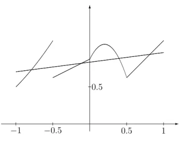
Figure 1.2: Data points and regression function.

piecewise polynomial:

m(x) =











(x+ 2)²/2 if −1≤x <−0.5, x/2 + 0.875 if −0.5≤x <0,

−5(x−0.2)²+ 1.075 if 0< x≤0.5, x+ 0.125 if 0.5≤x <1.

GivenX, the conditional distribution ofY−m(X)is normal with mean zero and standard deviation

σ(X) = 0.2−0.1 cos(2πX).

Figure 1.1 shows the data points. In this example the human eye is not able to see from the data points what the regression function looks like. In Figure 1.2 the data points are shown together with the regression function.

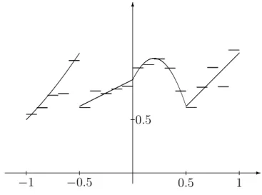
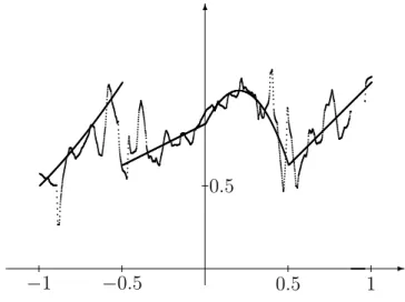
In Figure 1.3 a linear estimate is constructed for these simulated data. Obviously, a linear function does not approximate the regression function well.

Furthermore, for multivariate X, there is no easy way to visualize the data. Thus, especially for multivariateX, it is not clear how to choose a proper form of a parametric estimate, and a wrong form will lead to a bad estimate. This inflexibility concerning the structure of the regression function is avoided by so-called nonparametric regression estimates.

We will now define the modes of convergence of the regression estimates that we will study in this book.

(10)

- 6

−1 −0.5 0.5 1

0.5

Figure 1.3: Linear regression estimate.

The first and weakest property an estimate should have is that, as the sample size grows, it should converge to the estimated quantity, i.e., the error of the estimate should converge to zero for a sample size tending to infinity. Estimates which have this property are called consistent.

To measure the error of a regression estimate, we use the L₂ error Z

|m_n(x)−m(x)|²µ(dx).

The estimate mn depends on the data Dn, therefore the L2 error is a random variable.

We are interested in the convergence of the expectation of this random variable to zero as well as in the almost sure (a.s.) convergence of this random variable to zero.

Definition 1.1. A sequence of regression function estimates {mn} is called weakly consistent for a certain distribution of (X, Y), if

n→∞lim E Z

(mn(x)−m(x))²µ(dx)

= 0.

Definition 1.2. A sequence of regression function estimates {m_n} is called strongly consistent for a certain distribution of (X, Y), if

n→∞lim Z

(m_n(x)−m(x))²µ(dx) = 0 with probability one.

(11)

It may be that a regression function estimate is consistent for a certain class of distributions of (X, Y), but not consistent for others. It is clearly desirable to have estimates that are consistent for a large class of distributions. In the next chapters we are interested in properties of m_n that are valid for all distributions of (X, Y), that is, in distribution-free or universal properties. The concept of universal consistency is important in nonparametric regression because the mere use of a nonparametric estimate is normally a consequence of the partial or total lack of information about the distribution of (X, Y). Since in many situations we do not have any prior information about the distribution, it is essential to have estimates that perform well foralldistributions. This very strong requirement of universal goodness is formulated as follows:

Definition 1.3. A sequence of regression function estimates {m_n} is called weakly universally consistent if it is weakly consistent for all distributions of (X, Y) with E{Y²}<∞.

Definition 1.4. A sequence of regression function estimates {m_n} is called strongly universally consistent if it is strongly consistent for all distributions of (X, Y) with E{Y²}<∞.

We will later give many examples of estimates that are weakly and strongly universally consistent.

If an estimate is universally consistent, then, regardless of the true underlying distribution of(X, Y), theL₂ error of the estimate converges to zero for a sample size tending to infinity. But this says nothing about how fast this happens. Clearly, it is desirable to have estimates for which the L₂ error converges to zero as fast as possible.

To decide about the rate of convergence of an estimate m_n, we will look at the expectation of theL₂ error,

E Z

|m_n(x)−m(x)|²µ(dx). (1.4)

A natural question to ask is whether there exist estimates for which (1.4) converges to zero at some fixed, nontrivial rate for all distributions of(X, Y). Unfortunately, such estimates do not exist, i.e., for any estimate the rate of convergence may be arbitrarily slow. In order to get nontrivial rates of convergence, one has to restrict the class of distributions, e.g., by imposing some smoothness assumptions on the regression function.

(12)

1.2 How to Estimate a Regression Function?

In this section we describe two principles of nonparametric regression: local averaging and empirical error minimization.

Recall that the regression function is defined by a conditional expectation m(x) =E{Y |X=x}.

If xis an atom of X, i.e., P{X=x}>0 then the conditional expectation is defined by the conventional way:

E{Y |X=x}= E{Y I^{X=x}} P{X =x} ,

whereI^A denotes the indicator function of setA. In this definition one can estimate the numerator by

1 n

n

X

i=1

YiI^{Xi=x}, while the denominator’s estimate is

1 n

n

X

i=1

I^{Xi=x},

so the obvious regression estimate can be mn(x) =

Pn

i=1Y_iI^{Xi=x}

Pn

i=1I^{Xi=x}

.

In the general case ofP{X=x}= 0 we can refer to the measure theoretic definition of conditional expectation (cf. Appendix of Devroye, Györfi, and Lugosi [?]). However, this definition is useless from the point of view of statistics. One can derive an estimate from the property

E{Y |X=x}= lim

h→0

E{Y I^{{kX−xk≤h}}} P{kX−xk ≤h}

so the following estimate can be introduced:

m_n(x) = Pn

i=1Y_iI^{kXi−xk≤h}

Pn

i=1I^{kXi−xk≤h}

. This estimate is called naive kernel estimate.

(13)

We can generalize this idea by local averaging, i.e., estimation of m(x) is the average of those Y_i, whereX_i is “close” to x. Such an estimate can be written as

m_n(x) =

n

X

i=1

W_n,i(x)·Y_i,

where the weights W_n,i(x) = W_n,i(x,X₁, . . . ,X_n) ∈ R depend on X₁, . . . ,X_n. Usually the weights are nonnegative andW_n,i(x)is “small” if X_i is “far” from x.

Examples of such an estimates are the partitioning estimate, the kernel estimateand the k-nearest neighbor estimate.

For nonparametric regression estimation, the other principle is the empirical error minimization estimates, where there is a classF_nof functions, and the estimate is defined by.

m_n(·) = arg min

f∈Fn

(1 n

n

X

i=1

|f(X_i)−Y_i|² )

. (1.5)

Hence it minimizes the empirical L2 risk 1 n

n

X

i=1

|f(X_i)−Y_i|² (1.6)

over F_n. Observe that it doesn’t make sense to minimize (1.6) over all (measurable) functionsf, because this may lead to a function which interpolates the data and hence is not a reasonable estimate. Thus one has to restrict the set of functions over which one minimizes the empirical L₂ risk. Examples of possible choices of the setF_n are sets of piecewise polynomials or sets of smooth piecewise polynomials (splines). The use of spline spaces ensures that the estimate is a smooth function. An important member of least squares estimates is the generalized linear estimates. Let {φ_j}^∞_j=1 be real-valued functions defined onR^d and let Fn be defined by

F_n= (

f; f =

`n

X

j=1

c_jφ_j )

.

Then the generalized linear estimate is defined by mn(·) = arg min

f∈Fn

(1 n

n

X

i=1

(f(Xi)−Yi)² )

= arg min

c1,...,c_`n





 1 n

n

X

i=1

`n

X

j=1

c_jφ_j(X_i)−Y_i

!²



 .

(14)

- 6

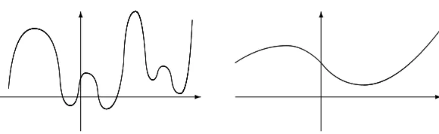
Figure 1.4: The estimate on the right seems to be more reasonable than the estimate on the left, which interpolates the data.

For least squares estimates, other example can be the neural networks or radial basis functions or orthogonal series estimates.

Letm_n be an arbitrary estimate. For anyx∈R^d we can write the expected squared error of mn at xas

E{|m_n(x)−m(x)|²}

=E{|m_n(x)−E{m_n(x)}|²}+|E{m_n(x)} −m(x)|²

=Var(m_n(x)) +|bias(m_n(x))|².

Here Var(mn(x)) is the variance of the random variable mn(x) and bias(mn(x)) is the difference between the expectation of m_n(x) and m(x). This also leads to a similar decomposition of the expected L₂ error:

E Z

|mn(x)−m(x)|²µ(dx)

= Z

E{|m_n(x)−m(x)|²}µ(dx)

= Z

Var(m_n(x))µ(dx) + Z

|bias(m_n(x))|²µ(dx).

The importance of these decompositions is that the integrated variance and the integrated squared bias depend in opposite ways on the wiggliness of an estimate. If one increases the wiggliness of an estimate, then usually the integrated bias will decrease, but the integrated variance will increase (so-called bias–variance tradeoff).

In Figure 1.5 this is illustrated for the kernel estimate, where one has, under some regularity conditions on the underlying distribution and for the naive kernel,

Z

R^d

Var(m_n(x))µ(dx) = c₁ 1 nh^d +o

1 nh^d

(15)

- 6

h Error

1 nh

h² 1

nh+h²

Figure 1.5: Bias–variance tradeoff.

and Z

R^d

|bias(m_n(x))|²µ(dx) = c₂h² +o h² .

Here h denotes the bandwidth of the kernel estimate which controls the wiggliness of the estimate,c₁ is some constant depending on the conditional varianceVar{Y|X=x}, the regression function is assumed to be Lipschitz continuous, and c₂ is some constant depending on the Lipschitz constant.

The value h^∗ of the bandwidth for which the sum of the integrated variance and the squared bias is minimal depends on c₁ and c₂. Since the underlying distribution, and hence also c₁ and c₂, are unknown in an application, it is important to have methods which choose the bandwidth automatically using only the data D_n.

(16)

(17)

Chapter 2 Partitioning Estimates

2.1 Introduction

In the next chapters we briefly review the most important local averaging regression estimates. Concerning further details see Györfiet al. [?].

LetP_n ={A_n,1, A_n,2, . . .} be a partition of R^d and for each x∈R^d letA_n(x)denote the cell of P_n containing x. The partitioning estimate (histogram) of the regression function is defined as

mn(x) = Pn

i=1Y_iI^{Xi∈An(x)}

Pn

i=1I^{Xi∈An(x)}

with0/0 = 0by definition. This means that the partitioning estimate is a local averaging estimate such for a givenxwe take the average of thoseY_i’s for which X_i belongs to the same cell into which xfalls.

The simplest version of this estimate is obtained for d = 1 and when the cells An,j

are intervals of size h = h_n. Figures 2.1 – 2.3 show the estimates for various choices of h for our simulated data introduced in Chapter 1. In the first figure h is too small (undersmoothing, large variance), in the second choice it is about right, while in the third it is too large (oversmoothing, large bias).

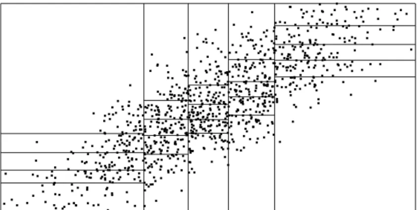
For d > 1 one can use, e.g., a cubic partition, where the cells A_n,j are cubes of volume h^d_n, or a rectangle partition which consists of rectangles A_n,j with side lengths h_n1, . . . , h_nd. For the sake of illustration we generated two-dimensional data when the actual distribution is a correlated normal distribution. The partition in Figure 2.4 is cubic, and the partition in Figure 2.5 is made of rectangles.

Cubic and rectangle partitions are particularly attractive from the computational point of view, because the set A_n(x) can be determined for each x in constant time,

(18)

- 6

−1 −0.5 0.5 1

0.5

Figure 2.1: Undersmoothing: h= 0.03, L₂ error =0.062433.

provided that we use an appropriate data structure. In most cases, partitioning estimates are computationally superior to the other nonparametric estimates, particularly if the search for A_n(x) is organized using binary decision trees (cf. Friedman [?]).

The partitions may depend on the data. Figure 2.6 shows such a partition, where each cell contains an equal number of points. This partition consists of so-called statistically equivalent blocks.

- 6

−1 −0.5 0.5 1

0.5

Figure 2.2: Good choice: h= 0.1, L₂ error =0.003642.

(19)

- 6

−1 −0.5 0.5 1

0.5

Figure 2.3: Oversmoothing: h= 0.5, L₂ error =0.013208.

Another advantage of the partitioning estimate is that it can be represented or com- pressed very efficiently. Instead of storing all dataD_n, one should only know the estimate for each nonempty cell, i.e., for cellsA_n,j for whichµ_n(A_n,j) >0, where µ_n denotes the empirical distribution. The number of nonempty cells is much smaller thann.

Figure 2.4: Cubic partition.

(20)

Figure 2.5: Rectangle partition.

2.2 Stone’s Theorem

In the next section we will prove the weak universal consistency of partitioning estimates.

In the proof we will use Stone’s theorem (Theorem 2.1 below) which is a powerful tool for proving weak consistency for local averaging regression function estimates. It will also be applied to prove the weak universal consistency of kernel and nearest neighbor estimates in Chapters 3 and 4.

Figure 2.6: Statistically equivalent blocks.

(21)

Local averaging regression function estimates take the form m_n(x) =

n

X

i=1

W_ni(x)·Y_i,

where the weightsW_n,i(x) = W_n,i(x,X₁, . . . ,X_n)∈R are depending on X₁, . . . ,X_n. Usually the weights are nonnegative and W_n,i(x) is “small” if X_i is “far” from x.

The next theorem states conditions on the weights which guarantee the weak universal consistency of the local averaging estimates.

Theorem 2.1. (Stone’s theorem). Assume that the following conditions are satisfied for any distribution of X:

(i) There is a constant c such that for every nonnegative measurable function f sat- isfying Ef(X)<∞ and any n,

E ( _n

X

i=1

|Wn,i(X)|f(Xi) )

≤cEf(X).

(ii) There is a D≥1 such that P

( _n X

i=1

|W_n,i(X)| ≤D )

= 1, for all n.

(iii) For all a >0,

n→∞lim E ( _n

X

i=1

|W_n,i(X)|I^{kXi−Xk>a}

)

= 0.

(iv)

n

X

i=1

Wn,i(X)→1 in probability.

(v)

n→∞lim E ( _n

X

i=1

W_n,i(X)² )

= 0.

(22)

Then the corresponding regression function estimatem_n is weakly universally consistent, i.e.,

n→∞lim E Z

(mn(x)−m(x))²µ(dx)

= 0 for all distributions of (X, Y) with EY² <∞.

For nonnegative weights and noiseless data (i.e., Y =m(X)≥ 0) condition (i) says that the mean value of the estimate is bounded above by some constant times the mean value of the regression function. Conditions (ii) and (iv) state that the sum of the weights is bounded and is asymptotically 1. Condition (iii) ensures that the estimate at a point x is asymptotically influenced only by the data close to x. Condition (v) states that asymptotically all weights become small.

One can verify that under conditions (ii), (iii), (iv), and (v) alone weak consistency holds if the regression function is uniformly continuous and the conditional variance functionσ²(x) is bounded. Condition (i) makes the extension possible. For nonnegative weights conditions (i), (iii), and (v) are necessary.

Definition 2.1. The weights{W_n,i}are called normal ifPn

i=1W_n,i(x) = 1. The weights {W_n,i}are called subprobability weights if they are nonnegative and sum up to≤1. They are called probability weights if they are nonnegative and sum up to 1.

Obviously for subprobability weights condition (ii) is satisfied, and for probability weights conditions (ii) and (iv) are satisfied.

2.3 Consistency

The purpose of this section is to prove theweakuniversal consistency of the partitioning estimates. This is the first such result that we mention. Later we will prove the same property for other estimates, too. The next theorem provides sufficient conditions for the weak universal consistency of the partitioning estimate. The first condition ensures that the cells of the underlying partition shrink to zero inside a bounded set, so the estimate is local in this sense. The second condition means that the number of cells inside a bounded set is small with respect ton, which implies that with large probability each cell contains many data points.

Theorem 2.2. If for each sphere S centered at the origin

n→∞lim max

j:An,j∩S6=∅diam(A_n,j) = 0 (2.1)

(23)

and

n→∞lim

|{j :A_n,j ∩S 6=∅}|

n = 0 (2.2)

then the partitioning regression function estimate is weakly universally consistent.

For cubic partitions,

n→∞lim h_n= 0 and lim

n→∞nh^d_n =∞ imply (2.1) and (2.2).

In order to prove Theorem 2.2 we will verify the conditions of Stone’s theorem. For this we need the following technical lemma. An integer-valued random variable B(n, p) is said to be binomially distributed with parameters n and 0≤p≤1if

P{B(n, p) = k}= n

k

p^k(1−p)^n−k, k = 0,1, . . . , n.

Lemma 2.1. Let the random variable B(n, p)be binomially distributed with parameters n and p. Then:

(i)

E

1 1 +B(n, p)

≤ 1

(n+ 1)p, (ii)

E 1

B(n, p)I{B(n,p)>0}

≤ 2

(n+ 1)p. Proof. Part (i) follows from the following simple calculation:

E

1 1 +B(n, p)

=

n

X

k=0

1 k+ 1

n k

p^k(1−p)^n−k

= 1

(n+ 1)p

n

X

k=0

n+ 1 k+ 1

p^k+1(1−p)^n−k

≤ 1

(n+ 1)p

n+1

X

k=0

n+ 1 k

p^k(1−p)^n−k+1

= 1

(n+ 1)p(p+ (1−p))ⁿ⁺¹

= 1

(n+ 1)p.

(24)

For (ii) we have

E 1

B(n, p)I{B(n,p)>0}

≤E

2 1 +B(n, p)

≤ 2

(n+ 1)p

by (i).

Proof of Theorem 2.2. The proof proceeds by checking the conditions of Stone’s theorem (Theorem 2.1). Note that if 0/0 = 0 by definition, then

W_n,i(x) =I^{Xi∈An(x)}/

n

X

l=1

I^{Xl∈An(x)}.

To verify (i), it suffices to show that there is a constant c > 0, such that for any nonnegative function f with Ef(X)<∞,

E ( _n

X

i=1

f(X_i) I^{Xi∈An(X)}

Pn

l=1I^{Xl∈An(X)}

)

≤cEf(X).

Observe that

E ( _n

X

i=1

Pn

l=1I^{Xl∈An(X)}

)

=

n

X

i=1

E (

1 +P

l6=iI^{Xl∈An(X)}

)

= nE (

f(X₁)I^{X1∈A_n(X)}

1 1 +P

l6=1I^{Xl∈An(X)}

)

= nE

E

f(X1)I^{X1∈An(X)}

1 1 +Pn

l=2I^{Xl∈An(X)}

X,X1

= nE

f(X1)I^{X1∈An(X)}E

1

1 +Pn

l=2I^{Xl∈An(X)}

X,X1

= nE

f(X1)I^{X1∈An(X)}E

1

1 +Pn

l=2I^{Xl∈An(X)}

X

(25)

by the independence of the random variables X,X₁, . . . ,X_n. Using Lemma 2.1, the expected value above can be bounded by

nE

f(X₁)I{X1∈An(X)}

1 nµ(A_n(X))

= X

j

P{X ∈A_nj} Z

Anj

f(u)µ(du) 1 µ(A_nj)

= Z

R^d

f(u)µ(du) = Ef(X).

Therefore, the condition is satisfied withc= 1. The weights are sub-probability weights, so (ii) is satisfied. To see that condition (iii) is satisfied first choose a ball S centered at the origin, and then by condition (2.1) a large n such that for A_n,j ∩S 6=∅ we have diam(A_n,j)< a. Thus X∈S and kX_i−Xk> aimply X_i ∈/ A_n(X), therefore

I{X∈S}

n

X

i=1

W_n,i(X)I{kXi−Xk>a}

= I^{X∈S}

Pn

i=1I^{Xi∈An(X),kX−X_ik>a}

nµ_n(A_n(X))

= I^{X∈S}

Pn

i=1I^{Xi∈A_n(X),Xi∈A/ _n(X),kX−X_ik>a}

nµ_n(A_n(X))

= 0.

Thus

lim sup

n E

n

X

i=1

W_n,i(X)I^{kXi−Xk>a} ≤µ(S^c).

(26)

Concerning (iv) note that P

( _n X

i=1

W_n,i(X)6= 1 )

= P{µ_n(A_n(X)) = 0}

= X

j

P{X∈A_n,j, µ_n(A_n,j) = 0}

= X

j

µ(A_n,j)(1−µ(A_n,j))ⁿ

≤ X

j:An,j∩S=∅

µ(An,j) + X

j:An,j∩S6=∅

µ(An,j)(1−µ(An,j))ⁿ. Elementary inequalities

x(1−x)ⁿ ≤xe^−nx ≤ 1

en (0≤x≤1) yield

P ( _n

X

i=1

Wn,i(X)6= 1 )

≤µ(S^c) + 1

en|{j :An,j∩S 6=∅}|.

The first term on the right-hand side can be made arbitrarily small by the choice of S, while the second term goes to zero by (2.2). To prove that condition (v) holds, observe

that n

X

i=1

W_n,i(x)² =

( ₁

Pn

l=1I{Xl∈An(x)} if µn(An(x))>0, 0 if µ_n(A_n(x)) = 0.

Then we have E

( _n X

i=1

W_n,i(X)² )

≤ P{X∈S^c}+ X

j:An,j∩S6=∅

E

I^{X∈An,j}

1

nµ_n(A_n,j)I^{µn(An,j)>0}

≤ µ(S^c) + X

j:An,j∩S6=∅

µ(A_n,j) 2 nµ(A_n,j) (by Lemma 2.1)

= µ(S^c) + 2

n |{j :A_n,j ∩S 6=∅}|.

(27)

A similar argument to the previous one concludes the proof.

2.4 Rate of Convergence

In this section we bound the rate of convergence ofEkmn−mk² for cubic partitions and regression functions which are Lipschitz continuous.

Theorem 2.3. For a cubic partition with side length h_n assume that Var(Y|X=x)≤σ², x∈R^d,

|m(x)−m(z)| ≤Ckx−zk,x,z∈R^d, (2.3) and thatX has a compact support S. Then

Ekm_n−mk² ≤ˆcσ²+ sup_z∈S|m(z)|²

n·h^d_n +d·C²·h²_n, where ˆc depends only on d and on the diameter of S, thus for

h_n=c⁰

σ²+ sup_z∈S|m(z)|² C²

1/(d+2)

n⁻^d+2¹

we get

Ekm_n−mk² ≤c⁰⁰

σ²+ sup

z∈S

|m(z)|²

2/(d+2)

C^2d/(d+2)n^−2/(d+2).

Proof. Set ˆ

m_n(x) =E{m_n(x)|X₁, . . . ,X_n}= Pn

i=1m(X_i)I^{Xi∈An(x)}

nµ_n(A_n(x)) . Then

E{(mn(x)−m(x))²|X1, . . . ,Xn}

= E{(m_n(x)−mˆ_n(x))²|X₁, . . . ,X_n}+ ( ˆm_n(x)−m(x))². (2.4)

(28)

We have

E{(m_n(x)−mˆ_n(x))²|X₁, . . . ,X_n}

= E

( Pn

i=1(Y_i−m(X_i))I^{Xi∈An(x)}

nµ_n(A_n(x))

²

X₁, . . . ,X_n )

= Pn

i=1Var(Y_i|X_i)I^{Xi∈An(x)}

(nµn(An(x)))²

≤ σ²

nµn(An(x))I{nµn(An(x))>0}.

By Jensen’s inequality

( ˆm_n(x)−m(x))² =

Pn

i=1(m(X_i)−m(x))I^{Xi∈A_n(x)}

nµ_n(A_n(x))

2

I^{nµn(An(x))>0}

+m(x)²I^{nµn(An(x))=0}

≤ Pn

i=1(m(X_i)−m(x))²I^{Xi∈An(x)}

nµ_n(A_n(x)) I^{nµn(An(x))>0}

+m(x)²I^{nµn(An(x))=0}

≤ d·C²h²_nI^{nµn(An(x))>0}+m(x)²I^{nµn(An(x))=0}

(by (2.3) and max

z∈A_n(x)kx−zk² ≤d·h²_n)

≤ d·C²h²_n+m(x)²I^{nµn(An(x))=0}.

Without loss of generality assume thatS is a cube and the union ofA_n,1, . . . , A_n,l_n is S.

Then

l_n ≤ ˜c h^d_n

(29)

for some constantc˜proportional to the volume of S and, by Lemma 2.1 and (2.4), E

Z

(m_n(x)−m(x))²µ(dx)

= E Z

(m_n(x)−mˆ_n(x))²µ(dx)

+E Z

( ˆm_n(x)−m(x))²µ(dx)

=

ln

X

j=1

E (Z

An,j

(m_n(x)−mˆ_n(x))²µ(dx) )

+

ln

X

j=1

E (Z

An,j

( ˆm_n(x)−m(x))²µ(dx) )

≤

ln

X

j=1

E

σ²µ(A_n,j)

nµ_n(A_n,j)I^{µn(An,j)>0}

+dC²h²_n

+

ln

X

j=1

E (Z

An,j

m(x)²µ(dx)I^{µn(An,j)=0}

)

≤

ln

X

j=1

2σ²µ(A_n,j)

nµ(A_n,j) +dC²h²_n+

ln

X

j=1

Z

An,j

m(x)²µ(dx)P{µ_n(A_n,j) = 0}

≤ l_n2σ²

n +dC²h²_n+ sup

z∈S

m(z)²

ln

X

j=1

µ(A_n,j)(1−µ(A_n,j))ⁿ

≤ l_n2σ²

n +dC²h²_n+l_nsup_z∈Sm(z)²

n sup

j

nµ(A_n,j)e^−nµ(A^n,j⁾

≤ l_n2σ²

n +dC²h²_n+l_nsup_z∈Sm(z)²e⁻¹ n

(since sup_zze^−z =e⁻¹)

≤ (2σ²+ sup_z∈Sm(z)²e⁻¹)˜c

nh^d_n +dC²h²_n.

(30)

(31)

Chapter 3 Kernel Estimates

3.1 Introduction

The kernel estimate of a regression function takes the form

m_n(x) = Pn

i=1Y_iK

x−Xi

hn

Pn

i=1K

x−Xi

hn

,

if the denominator is nonzero, and 0 otherwise. Here the bandwidth h_n > 0 depends only on the sample size n, and the function K : R^d → [0,∞) is called a kernel. (See Figure 3.1 for some examples.) Usually K(x) is “large” if kxk is “small,” therefore the kernel estimate again is a local averaging estimate.

Figures 3.2–3.5 show the kernel estimate for the naive kernel (K(x) = I{kxk≤1}) and for the Epanechnikov kernel (K(x) = (1− kxk²)₊) using various choices for h_n for our simulated data introduced in Chapter 1.

Figure 3.6 shows the L₂ error as a function of h.

- 6

K(x) =I{||x||≤1}

x ^-

6

K(x) = (1−x²)₊

x ^-

6K(x) = e^−x²

x

Figure 3.1: Examples for univariate kernels.

(32)

- 6

−1 −0.5 0.5 1

0.5

Figure 3.2: Kernel estimate for the naive kernel: h= 0.1, L₂ error =0.004066.

3.2 Consistency

In this section we use Stone’s theorem (Theorem 2.1) in order to prove the weak universal consistency of kernel estimates under general conditions on h and K.

Theorem 3.1. Assume that there are balls S_0,r of radius r and balls S_0,R of radius R

- 6

−1 −0.5 0.5 1

0.5

Figure 3.3: Undersmoothing for the Epanechnikov kernel: h= 0.03,L₂error =0.031560.

(33)

- 6

−1 −0.5 0.5 1

0.5

Figure 3.4: Kernel estimate for the Epanechnikov kernel: h= 0.1,L₂ error = 0.003608.

centered at the origin (0< r≤R), and constant b >0 such that I^{x∈S0,R} ≥K(x)≥bI^{x∈S0,r}

(boxed kernel), and consider the kernel estimate m_n. If h_n →0 and nh^d_n → ∞, then the kernel estimate is weakly universally consistent.

As one can see in Figure 3.7, the weak consistency holds for a bounded kernel with compact support such that it is bounded away from zero at the origin. The bandwidth must converge to zero but not too fast.

Proof. Put

K_h(x) =K(x/h).

We check the conditions of Theorem 2.1 for the weights W_n,i(x) = K_h(x−X_i)

Pn

j=1K_h(x−X_j). Condition (i) means that

E (Pn

i=1K_h(X−X_i)f(X_i) Pn

j=1Kh(X−Xj) )

≤cE{f(X)}

(34)

with c >0. Because of

E (Pn

i=1K_h(X−X_i)f(X_i) Pn

j=1K_h(X−X_j) )

= nE

(K_h(X−X₁)f(X₁) Pn

j=1K_h(X−X_j) )

= nE

( K_h(X−X₁)f(X₁) K_h(X−X₁) +Pn

j=2K_h(X−X_j) )

= n Z

f(u)

"

E (Z

Kh(x−u) K_h(x−u) +Pn

j=2K_h(x−X_j)µ(dx) )#

µ(du)

it suffices to show that, for all u and n,

E

(Z K_h(x−u) K_h(x−u) +Pn

j=2K_h(x−X_j)µ(dx) )

≤ c n.

The compact support of K can be covered by finitely many balls, with translates of S_0,r/2, where r >0is the constant appearing in the condition on the kernel K, and with

- 6

−1 −0.5 0.5 1

0.5

Figure 3.5: Oversmoothing for the Epanechnikov kernel: h= 0.5,L₂ error = 0.012551.

(35)

- 6

0.1 0.2

0.1 0.25 h

Error

Figure 3.6: The L₂ error for the Epanechnikov kernel as a function ofh.

centers x_i, i= 1,2, . . . , M. Then, for all x and u,

K_h(x−u)≤

M

X

k=1

I^{x∈u+hxk+S_0,rh/2}.

Furthermore,x∈u+hxk+S0,rh/2 implies that

u+hx_k+S_0,rh/2 ⊂x+S_0,rh

- 6K(x)

x 1

b

−r r

−R R

Figure 3.7: Boxed kernel.

(36)

x r

z

r 2

Figure 3.8: If x∈S_z,r/2, then S_z,r/2 ⊆S_x,r. (cf. Figure 3.8). Now, by these two inequalities,

E (Z

K_h(x−u) K_h(x−u) +Pn

≤

M

X

k=1

E (Z

u+hxk+S_0,rh/2

K_h(x−u) K_h(x−u) +Pn

≤

M

X

k=1

E (Z

u+hxk+S0,rh/2

1 1 +Pn

j=2Kh(x−Xj)µ(dx) )

≤ 1 b

M

X

k=1

E (Z

u+hxk+S_0,rh/2

1 1 +Pn

j=2I^{Xj∈x+S_0,rh}

µ(dx) )

≤ 1 b

M

X

k=1

E (Z

u+hxk+S_0,rh/2

1 1 +Pn

j=2I^{Xj∈u+hx_k+S_0,rh/2}

µ(dx) )

= 1 b

M

X

k=1

E

( µ(u+hx_k+S_0,rh/2) 1 +Pn

j=2I^{Xj∈u+hx_k+S_0,rh/2}

)

≤ 1 b

M

X

k=1

µ(u+hxk+S_0,rh/2) nµ(u+hx_k+S_0,rh/2) (by Lemma 2.1)

≤ M nb.

(37)

The condition (ii) holds since the weights are subprobability weights.

Concerning (iii) notice that, for h_nR < a,

n

X

i=1

|W_n,i(X)|I^{kXi−Xk>a} = Pn

i=1Khn(X−Xi)I^{kXi−Xk>a}

Pn

i=1K_h_n(X−X_i) = 0.

In order to show (iv), mention that 1−

n

X

i=1

W_n,i(X) = I{^Pⁿi=1K_hn(X−X_i)=0}, therefore,

P (

16=

n

X

i=1

Wn,i(X) )

= P ( _n

X

i=1

Khn(X−Xi) = 0 )

≤ P ( _n

X

i=1

I^{Xi6∈S_X,rhn} = 0 )

= P{µ_n(S_X,rh_n) = 0}

= Z

(1−µ(S_x,rh_n))ⁿµ(dx).

Choose a sphereS centered at the origin, then P

( 16=

n

X

i=1

W_n,i(X) )

≤ Z

S

e^−nµ(S^x,rhn⁾µ(dx) +µ(S^c)

= Z

S

nµ(S_x,rh_n)e^−nµ(S^x,rhn⁾ 1

nµ(S_x,rh_n)µ(dx) +µ(S^c)

= max

u ue^−u Z

S

1

nµ(S_x,rh_n)µ(dx) +µ(S^c).

By the choice of S, the second term can be small. For the first term we can find z₁, . . . ,z_M_n such that the union of S_z₁_,rh_n_/2, . . . , S_z_Mn_,rh_n_/2 covers S, and

M_n≤ c˜ h^d_n.

(38)

Then

Z

S

1

nµ(S_x,rh_n)µ(dx) ≤

Mn

X

j=1

Z I^{x∈Szj ,rhn/2}

nµ(S_x,rh_n) µ(dx)

≤

Mn

X

j=1

Z I^{x∈Szj ,rhn/2}

nµ(S_z_j_,rh_n_/2)µ(dx)

≤ M_n n

≤ ˜c

nh^d_n →0. (3.1)

Concerning (v), since K(x)≤1we get that, for any δ >0,

n

X

i=1

Wn,i(X)² =

Pn

i=1K_h_n(X−X_i)² (Pn

i=1K_h_n(X−X_i))²

≤

Pn

i=1K_h_n(X−X_i) (Pn

i=1K_h_n(X−X_i))²

≤ min

δ, 1

Pn

i=1K_h_n(X−X_i)

≤ min

δ, 1

Pn

i=1bI^{Xi∈S_X,rhn}

≤ δ+ 1

Pn

i=1bI^{Xi∈S_X,rhn}Iⁿ^Pⁿ

i=1I{Xi∈SX,rhn}>0o,

therefore it is enough to show that

E

1 Pn

i=1I^{Xi∈S_X,rhn}Iⁿ^Pⁿ

i=1I{Xi∈SX,rhn}>0o

→0.

(39)

LetS be as above, then E

1 Pn

i=1I{Xi∈SX,rhn}>0 o

≤ E

1 Pn

i=1I{Xi∈SX,rhn}>0

oI^{X∈S}

+µ(S^c)

≤ 2E

1

(n+ 1)µ(S_X,h_n)I^{X∈S}

+µ(S^c) (by Lemma 2.1)

→ µ(S^c)

as above.

3.3 Rate of Convergence

In this section we bound the rate of convergence of Ekm_n−mk² for a naive kernel and a Lipschitz continuous regression function.

Theorem 3.2. For a kernel estimate with a naive kernel assume that Var(Y|X=x)≤σ², x∈R^d,

and

|m(x)−m(z)| ≤Ckx−zk,x,z∈R^d, and X has a compact support S^∗. Then

Ekm_n−mk² ≤ˆcσ²+ sup_z∈S∗|m(z)|²

n·h^d_n +C²h²_n, where ˆc depends only on the diameter of S^∗ and on d, thus for

h_n=c⁰

σ²+ sup_z∈S^∗|m(z)|² C²

1/(d+2)

n⁻^d+2¹ we have

Ekm_n−mk² ≤c⁰⁰

σ² + sup

z∈S^∗

|m(z)|²

2/(d+2)

C^2d/(d+2)n^−2/(d+2).

Nonparametric Statistics