IstvánHegedűs ,GáborDanner ,MárkJelasity Decentralizedlearningworks:Anempiricalcomparisonofgossiplearningandfederatedlearning J.ParallelDistrib.Comput.

Contents lists available atScienceDirect

J. Parallel Distrib. Comput.

journal homepage:www.elsevier.com/locate/jpdc

Decentralized learning works: An empirical comparison of gossip learning and federated learning

István Hegedűs

, Gábor Danner

, Márk Jelasity

aUniversity of Szeged, Szeged, Hungary

bMTA SZTE Research Group on Artificial Intelligence, Szeged, Hungary

a r t i c l e i n f o

Article history:

Received 15 October 2019

Received in revised form 8 October 2020 Accepted 18 October 2020

Available online 4 November 2020

Keywords:

Federated learning Gossip learning

Decentralized machine learning

a b s t r a c t

Machine learning over distributed data stored by many clients has important applications in use cases where data privacy is a key concern or central data storage is not an option. Recently, federated learning was proposed to solve this problem. The assumption is that the data itself is not collected centrally. In a master–worker architecture, the workers perform machine learning over their own data and the master merely aggregates the resulting models without seeing any raw data, not unlike the parameter server approach. Gossip learning is a decentralized alternative to federated learning that does not require an aggregation server or indeed any central component. The natural hypothesis is that gossip learning is strictly less efficient than federated learning due to relying on a more basic infrastructure: only message passing and no cloud resources. In this empirical study, we examine this hypothesis and we present a systematic comparison of the two approaches. The experimental scenarios include a real churn trace collected over mobile phones, continuous and bursty communication patterns, different network sizes and different distributions of the training data over the devices. We also evaluate a number of additional techniques including a compression technique based on sampling, and token account based flow control for gossip learning. We examine the aggregated cost of machine learning in both approaches. Surprisingly, the best gossip variants perform comparably to the best federated learning variants overall, so they offer a fully decentralized alternative to federated learning.

©2020 The Author(s). Published by Elsevier Inc. This is an open access article under the CC BY license (http://creativecommons.org/licenses/by/4.0/).

1. Introduction

Performing data mining over data collected by edge devices, most importantly, mobile phones, is of very high interest [34].

Collecting such data at a central location has become more and more problematic in the past years due to novel data protection rules [1] and in general due to the increasing public awareness to issues related to data handling. For this reason, there is an increasing interest in methods that leave the raw data on the device and process it using distributed aggregation.

Google introduced federated learning to answer this chal- lenge [22,25]. This approach is very similar to the well-known parameter server architecture for distributed learning [11] where worker nodes store the raw data. The parameter server maintains the current model and regularly distributes it to the workers who

✩ This work was supported by the Hungarian Government and the European Regional Development Fund under the grant number GINOP-2.3.2-15-2016- 00037 (‘‘Internet of Living Things’’), by grant TUDFO/47138-1/2019-ITM of the Ministry for Innovation and Technology, Hungary, and by the University of Szeged Open Access Fund, Hungary (Grant Number 4411).

∗ Corresponding author at: University of Szeged, Szeged, Hungary.

E-mail address: jelasity@inf.u-szeged.hu(M. Jelasity).

in turn calculate a gradient update and send it back to the server.

The server then applies all the updates to the central model.

This is repeated until the model converges. In federated learning, this framework is optimized so as to minimize communication between the server and the workers. For this reason, the local update calculation is more thorough, and compression techniques can be applied when uploading the updates to the server.

In addition to federated learning,gossip learninghas also been proposed to address the same challenge [15,27]. This approach is fully decentralized, no parameter server is necessary. Nodes exchange and aggregate models directly. The advantages of gossip learning are obvious: since no infrastructure is required, and there is no single point of failure, gossip learning enjoys a sig- nificantly cheaper scalability and better robustness. A key ques- tion, however, is how the two approaches compare in terms of performance. This is the question we address in this work.

We compare the two approaches in terms of convergence time and model quality, assuming that both approaches utilize the same amount of communication resources in the same sce- narios. In other words, we are interested in the question of whether—by communicating the same number of bits in the same time-window—the two approaches can achieve the same model quality. We train linear models using stochastic gradient descent

https://doi.org/10.1016/j.jpdc.2020.10.006

0743-7315/©2020 The Author(s). Published by Elsevier Inc. This is an open access article under the CC BY license (http://creativecommons.org/licenses/by/4.0/).

(SGD)

based on the logistic regression loss function.

Our experimental methodology involves several scenarios, in- cluding smartphone churn traces collected by the application Stunner [5]. We also vary the communication pattern (continuous or bursty) and the network size. In addition, we also evaluate dif- ferent assumptions about the label distribution, that is, whether a given worker has a biased or unbiased subset of the training samples.

To make the comparison as fair as possible, we make sure that the two approaches differ mainly in their communication pat- terns. However, the computation of the local update is identical in both approaches. Also, we apply subsampling to reduce commu- nication in both approaches, as introduced in [22] for federated learning. Here, we adapt the same technique for gossip learning.

We also introduce a token account based flow control mechanism for gossip learning, for the case of bursty communication.

We note that both approaches offer mechanisms for explicit privacy protection, apart from the basic feature of not collecting data. In federated learning, Bonawitz et al. [7] describe a secure aggregation protocol, whereas for gossip learning one can apply the methods described in [8]. Here, we are concerned only with the efficiency of the different communication patterns and we do not compare security mechanisms.

The result of our comparison is that gossip learning is in gen- eral comparable to the centrally coordinated federated learning approach. This result is rather counter-intuitive and suggests that decentralized algorithms should be treated as first class citizens in the area of distributed machine learning overall, considering the additional advantages of decentralization.

This paper is a thoroughly revised and extended version of a conference publication [16]. The novel contributions relative to this conference publication are:

• A new evaluation scenario involving bursty traffic, in which nodes communicate in high bandwidth bursts. This is a very different scenario from continuous communication be- cause here, it is possible to have fast ‘‘hot potato’’ chains of messages without increasing average bandwidth.

• The presentation and evaluation of a novel application of a token based flow control mechanism for gossip learning in the bursty transfer scenario.

• The introduction of a new subsampling technique based on partitioned models where each partition has its own age parameter. We show that this partitioning technique is beneficial for token-based learning algorithms.

• New experimental scenarios including larger networks, and an additional variant of compressed federated learning where the downstream traffic is also compressed using subsampling.

• A thorough hyperparameter analysis in Section5.4.

The outline is as follows. Sections 2–4 describe the basics of logistic regression, gossip learning, and federated learning, respectively. These sections describe our novel algorithms as well, including the token account based flow control mechanism, the model partitioning technique, and a number of smaller design decisions that allow all the evaluated algorithms to use shared components. Section5presents our experimental setup that in- cludes the applied datasets, as well as our system model. We also discuss the problem of selecting hyperparameters. Section6 describes our experimental results in a large number of scenarios with many algorithm variants. Section 7 presents related work and Section8concludes the paper.

2. Machine learning basics

Here, we give a concise summary of the main machine learn- ing concepts. We are concerned with the classification problem, where we are given a data setD = {(x₁,^y1), . . . ,^(xn,^yn)} ofn examples. An example (x,y) consists of a feature vectorx ∈ R^d and the corresponding class labely∈C, wheredis the dimension of the problem andC is the set of class labels.

The problem is to find the parametersw of a functionf_w : R^d→C that can correctly classify as many examples as possible inD, as well as outsideD(this latter property is called general- ization). Expressed formally, we wish to minimize an objective functionJ(w^{) in}w^:

w^∗=arg min

w J(w⁾=arg min

w

1 n

n

∑

i=₁

ℓ^(fw(x_i),^yi)+λ

2∥w∥², ⁽¹⁾ whereℓ() is the loss function (the error of the prediction),∥w∥² is the regularization term, andλis the regularization coefficient.

Stochastic gradient descent (SGD) is a popular approach for findingw^∗. Here, we start with some initial weight vectorw0, and we apply the following update rule:

wt+₁=wt−ηt(λwt+∂ℓ^(fw(x_i),^yi)

∂w ⁽wt)). ⁽²⁾

Here, ηt is called the learning rate. This update rule requires a single example (x_i,^yi), and in each update we can choose a random example.

In this study we uselogistic regressionas our machine learning model, where the specific form of the objective function is given by

J(w,^b)= λ

2∥w∥²−¹ n

n

∑

i=₁

[y_ilnf_(w,b)(x_i)+(1−y_i)

× ln(1−f_(w,b)(x_i))]

, ⁽³⁾

wherey_i∈ {0,¹}and

f_(w,b)(x_i)=P(y_i=1|x_i, w,^b)= ¹

1+e^(wTx+b). ⁽⁴⁾ Note that P(y_i = 0|x_i, w,^b) = 1−P(y_i = 1|x_i, w,b). In fact, the loss function above is the log-likelihood of the data under this probabilistic model. The parameterbis called the bias of the model.

While our method can be applied to solve any model-fitting optimization problem, we evaluated it only with logistic regres- sion. This might seem restrictive, however, the practical applica- bility of such a simple linear model is greatly extended if one uses it in the context of transfer learning [31]. The idea is that arbitrarily complex pre-trained machine learning models are used as feature extractors, over which a simple (often linear) model is trained over a given new dataset. In linguistic applications, this is becoming a very popular approach, often using BERT [12] as the pre-trained model. This can approximate the performance of training the entire complex model over the new dataset, while using much fewer resources.

3. Gossip learning

Gossip Learning is a machine learning approach over fully distributed data without central control [27]. Here, we assume that the data setDis horizontally distributed over a set of nodes, with nodekstoring its own shardD_k. The task is to collectively find a machine learning model in such a way that it emulates the case when the data set is stored centrally.

Let us discuss the basic notions of gossip learning. Each node k runs Algorithm 1. First, the node initializes its local model

Algorithm 1Gossip Learning

1: (t_k, wk,^bk)←(0,⁰,⁰⁾

2: loop

3: wait(∆g)

4: p←selectPeer()

5: send sample(t_k, wk,^bk) top

6: end loop

7:

8: procedureonReceiveModel(t_r, wr,^br)

9: (t_k, wk,^bk)←merge((t_k, wk,^bk),^(tr, wr,^br))

10: (t_k, wk,^bk)←update((t_k, wk,^bk),^Dk)

11: end procedure

(wk,^bk) and its age t_k. A subset of the model parameters is then periodically sent to another node in the network. When a node receives such a parameter sample, it merges it into its own model and then it performs a local update step. Note that the rounds are not synchronized, although all the nodes use the same period ∆g. Any received messages are processed immediately.

Different variants of the algorithm can be produced with different implementations of the methods _sample, _merge, and _update. In the simplest case, samplesends the entire model (no sampling), mergecomputes the average, andupdateperforms a mini-batch update based on the local data. Later on, we will define more sophisticated implementations in Section3.1.

The node selection in line4is supported by a so-called peer sampling service. Applications can utilize a peer sampling service implementation to obtain random samples from the set of partici- pating nodes. The implementations of this service might be based on several different approaches that include random walks [32], gossip [19], or even static overlay networks that are created at random and repaired when necessary [28]. We will assume a static, connected, random overlay network from now on.

In the following, we shall describe three optimizations of the original gossip learning algorithm, that are interrelated. Very briefly, the basic ideas behind the three optimizations are the following:

sampling: Instead of sending the full model to the neighbor, a node can send only a subset of the parameters. This technique is often used as a compression mechanism to save bandwidth.

model partitioning: Related to sampling, instead of a random subset, it is also possible to define a fixed partitioning of the model parameters and to send one of these subsets as a sample.

token accounts [10]: We can add flow control as well, that is, we can speed up the spreading of information through a self-organizing enhancement of the communication pat- tern, without increasing the number of messages overall.

These three techniques are interrelated. For example, if one wishes to use token accounts along with sampling-based com- pression, then using the implementation based on model par- titioning is imperative, as we will see. In fact, that is our main motivation for discussing model partitioning. Let us now discuss these techniques in turn.

3.1. Random sampling and model partitioning

As for the methodsample, we will use two different implemen- tations. The first implementation, sampleRandom(t, w,^b,^{s) re-} turns a uniform random subset of the parameters, where

Algorithm 2Partitioned Model Merge

1: S:the number of partitions

2: proceduremerge((t, w,^b),^(tr, wr,^br))

3: j←index of received partition ▷j=i modS, for any coordinateiwithin the sample

4: forcoordinateiis included in sampledo

5: w[i] ←(t[j] ·w[i] +t_r[j] ·wr[i])/^(t[j] +t_r[j])

6: end for

7: b←(t[S] ·b+t_r[S] ·b_r)/^(t[S] +t_r[S])

8: t←max(t,^tr) ▷element-wise maximum, wheret_r is defined

9: return(t, w,^b)

10: end procedure

s ∈(0,¹]defines the size of the sample. To be precise, the size of the sample is given bys·d(randomly rounded) wheredis the dimension of vectorw^.

The other implementation is based on a partitioning of the model parameters. Let us elaborate on the idea of model parti- tioning here. The model is formed by the vectorwand the bias value b. We partition only w. We define S ≥ 1 partitions, by assigning a given vector indexito the partition index (i modS).

When sampling is based on this partitioning, we return a given partition. More precisely, samplePartition(t, w,^b,j), where 0 ≤ j<^Sis a partition index, returns partitionj. The biasbis always included in every sample, in both implementations of method sample.

It is important to stress that the random sampling method sampleRandomshould be applied only without model partitioning (that is, whenS = 1). It is possible to define a combination of partition-based and random sampling, where we could sample from a given partition, but we do not explore this possibility in this study.

Upon receiving a model, the node merges it with its local model, and updates it using its local data setD_k. Method_mergeis used to combine the local model with the incoming one. The most usual choice to implement mergeis to take the average of the parameter vectors [27]. This is supported by theoretical findings as well, at least in the case of linear models and when there is only one round of communication [35].

If there is no partitioning (S = 1) then the implementation shown as Algorithm2computes the average weighted by model age. This implementation can deal with subsampled input as well, since we consider only those parameters that are actually included in the sample. When partitioning is applied (that is, when S > 1) each partition of the parameter vector has its own age parameter. This is crucial especially when we apply flow control to speed up communication, as we explain later on. This means that every model now has a vector of age valuestof length S+1 where the ages of the partitions aret[0], . . . ,^t[S−1]and the age of the bias ist[S].

Method_updateis shown in Algorithm3. This implementation requires a full model as input but it does take into account the partitioning of the model in that all the partitions have their own dynamic learning rate that is determined by the age of the partition.

3.2. Token gossip learning

In our previous work, we introduced the token account algo- rithm for improving the efficiency of gossip protocols in a wide range of applications [10]. The basic intuition is that the token account algorithm allows chains of messages to form that travel fast in the network like a ‘‘hot potato’’, even if the budget of

111

Algorithm 3Partitioned Model Update Rule

1: S:the number of partitions

2: d:the dimension ofw

3: procedureupdate((t, w,^b),^D)

4: for allbatchB⊆Ddo ▷D is split into batches

5: t←t+ |B|·1 ▷increase all ages by|B|

6: fori∈ {1, ...,^d}do

7: h[i] ← − η

t[i modS]

∑

(x,y)∈_B

(∂ℓ^(fw,b(x),^y)

∂w[i] ⁽w[i]) + λw[i])

8: end for

9: g← − η

t[S]

∑

(x,y)∈_B

(∂ℓ^(fw,b(x),^y)

∂^{b (b)}+λ^b)

10: w←w+h

11: b←b+g

12: end for

13: return(t, w,^b)

14: end procedure

Algorithm 4Partitioned Token Gossip Learning

1: (t_k, wk,^bk)←(0,⁰,⁰⁾

2: a_k←0

3: loop

4: wait(∆g)

5: j←selectPart() ▷select a random partition

6: do with probabilityproactive(a_k[j])

7: p←selectPeer()

8: send samplePartition(t_k, wk,^bk,^{j) top}

9: else

10: a_k[j] ←a_k[j] +1 ▷we did not spend the token so it accumulates

11: end do

12: end loop

13:

14: procedureonReceiveModel(t_r, wr,^br,^j)

15: (tk, wk,^bk)←merge((tk, wk,^bk),^(tr, wr,^br))

16: (t_k, wk,^bk)←update((t_k, wk,^bk),^Dk)

17: x←randRound(reactive(a_k[j]))

18: a_k[j] ←a_k[j] −x ▷we spendxtokens

19: fori←1 toxdo

20: p←selectPeer()

21: send samplePartition(t_k, wk,^bk,^{j) top}

22: end for

23: end procedure

each node is limited. This is due to the flow control mechanism implemented with the help of token accounts that allow these hot potatoes to avoid waiting for the next cycle at each node. So far, the token account approach has not been applied to merge-based gossip learning. Here, we omit the general introduction of the entire family of token account algorithms and instead we focus on the novel variant that is applicable in this study, shown as Algorithm4.

It is very important that the algorithm uses samplePartition as an implementation of sampling. Our preliminary experiments have shown that random sampling (sampleRand) is not effective along with the token account technique. This is because if we sample independently at each hop, we work strongly against the formation of long ‘‘hot potato’’ message chains that represent any fixed model parameter. This is a key insight, and this is why the partitioned approach is expected to work better. It allows for hot potato message chains to form based on a single partition.

In other words, we can have the benefits of sampling-based compression and hot potato message passing at the same time.

Accordingly, each partitionjat nodeknow has its own token accounta_k[j]that stores the number of available tokens. Apart from the flow control extension, the algorithm is very similar to general gossip learning. The main difference is that we might also send messages reactively, that is, as a direct reaction to receiving a model. The only two methods that we need to define are proactiveand_reactive. Method_proactivereturns the probability of sending a proactive message as a function of the number of tokens. Methodreactivereturns the number of reactive messages to be sent. Here, we used the implementations

proactive(a)=

⎧

⎨

⎩

0 if a<^A−1 a−A+1

C−A+1 if a∈ [A−1,^C] ⁽⁵⁾ andreactive(a)=a/A, with parametersA=10 andC=20, based on our previous work [10]. Here,C >0 is the maximal number of tokens the account can store. Note that the maximum value of ais indeedCbecause initiallya=0 and whena=C, we always send a proactive message, thusawill not grow further. Parameter A∈ {1, . . . ,^C}plays a role in both reactive and proactive message sending, and it can be interpreted as the motivation level for saving tokens. IfA=1, then we spend all our tokens on sending reactive messages in every call to onReceiveModel and we also send proactive messages with a positive probability if the account is not empty. IfA=Cthen we send at most one reactive message, and we send a proactive message only if the account is full.

With each partition having a separate account, each partition will perform random walks independently, using its own commu- nication budget. Of course, the model update is not independent, it is the same as in partitioned gossip learning. We also track the age of each partition, as discussed previously in connection with the merge and update functions. We will argue that even plain gossip learning can benefit from using partitions, although to a lesser extent.

If the number of partitions isS=1, then we get a special case of the algorithm without any compression (that is, no sampling), we always send the entire model.

As a final note, let us mention that the methodsselectPartand selectPeer were implemented using sampling without replace- ment, re-initialized when the pool of available options becomes empty. This is slightly better than sampling with replacement, because it results in a lower variance.

4. Federated learning

Federated learning is not a specific algorithm, but more of a design framework for edge computing. We discuss federated learning based on the algorithms presented in [22,25]. While we keep the key design elements, our presentation contains small ad- justments and modifications to accommodate our contributions and to allow gossip learning and federated learning to share a number of key methods.

The pseudocode of the federated learning algorithm is shown in Algorithms5(master) and6(worker). The master periodically sends the current modelwto all the workers asynchronously in parallel and collects the answers from the workers. In this version of the algorithm, communication is compressed through sampling the parameter vectors. The rate of sampling might be different in the case of downstream messages (line4of Algorithm5) and up- stream messages (line11of Algorithm6). We require thats_up≤ s_down. Although this is not reflected in the pseudocode for pre- sentation clarity, the sample produced in line11of Algorithm6 is allowed to include only indices that are also included in the

Algorithm 5Federated Learning Master

1: (t, w,^b)←init()

2: loop

3: forevery nodekin parallel do ▷non-blocking (in separate threads)

4: send sample(t, w,^b,^sdowⁿ) tok

5: receive (n_k,^hk,^gk) fromk ▷n_k: #examples atk;h_k: sampled model gradient;g_k: bias gradient

6: end for

7: wait(∆f) ▷the round length

8: n← _|¹

K|

∑

k∈Kn_k ▷K: nodes that returned a model in this round

9: t ←t+n

10: h←aggregate({h_k:k∈K})

11: w←w+h

12: g ← _|K¹_|∑

k∈Kgk 13: b←b+g

14: end loop

Algorithm 6Federated Learning Worker

1: (t_k, wk,^bk)←init() ▷the local model at the worker

2:

3: procedureonReceiveModel(t, w,^b) ▷w: sampled model

4: t_k←t

5: forw[i] ∈w^do ▷coordinateiis defined inw

6: wk[i] ←w[i]

7: end for

8: b_k←b

9: (t_k, wk,^bk)←update((t_k, wk,^bk),^Dk) ▷D_k: the local database of examples

10: (n,^h,^g)←(t_k−t, wk−w,^bk−b) ▷n: the number of local examples,h: the gradient update

11: send sample(n,^h,^g,^sup) to master

12: end procedure

Algorithm 7Variants of the aggregate function

1: procedureaggregate(H)

2: h^′←0

3: fori∈ {1, ...,^d}do

4: h^′[i] ←_s|¹_H|∑

h∈_H:_h[_i]∈_hh[i] ▷s∈(0,¹]: sampling rate used to createH

5: end for

6: returnh^′

7: end procedure

8:

9: procedureaggregateImproved(H)

10: h^′←0

11: fori∈ {1, ...,^d}do

12: H_i← {h:h∈H∧h[i] ∈h}

13: h^′[i] ← ¹

|_Hi|₍₁−₍₁−_s)^|H|₎

∑

h∈_Hih[i] ▷skipped if|H_i|=0

14: end for

15: returnh^′

16: end procedure

received model. For example, if s_up = s_down then the worker selects exactly those indices that were received in the incoming sample.

Any answers from workers arriving with a delay larger than

∆f are simply discarded. After∆f time units have elapsed, the master aggregates the received gradients and updates the model.

We also send and maintain the model aget (based on the aver- age number of examples used for training) in a similar fashion, to make it possible to use dynamic learning rates in the local learning algorithm.

We note that, although in this version of the algorithm the master sends the model to every worker, it is possible to use a more fine-grained method to select a subset of workers that get the model in a given round. For example, if the workers have a very limited budget of communication, it might be better to avoid talking to each worker in each round. Indeed, we will study such a scenario during our experimental evaluation, but we did not want to include this option in the pseudocode for clarity of presentation.

These algorithms are very generic, the key characteristics of federated learning lie in the details of the update method (line9of Algorithm6) and the aggregation mechanism (line10 of Algorithm 5). The update method is typically implemented through a minibatch gradient descent algorithm that operates on the local data, initialized with the received model w^{. The} implementation we use here is identical to that of gossip learning, as given in Algorithm3. Note that here we do not partition the model (that is,S =1). As for sampling, we usesampleRandomas described in Section3.1.

Method aggregate is used in Algorithm5. Its function is to aggregate the received sampled gradients. Possible implemen- tations are shown in Algorithm 7. Both implementations are unbiased estimates of the average gradient. This also implies that when there is no actual sampling (that is, we haves = 1) then simply the average of the gradients is computed by both methods.

The improved version averages each coordinate separately, that is, it takes the average of only those coordinates that are included in the sample. This is a more accurate estimate of the true average of the given coordinate. However, in order to get an unbiased estimate, we have to divide by the probability that there is at least one gradient in which the given coordinate is included. This probability equals 1−(1− s)^|H|. Note that this probability is independent of the coordinatei, so its effect can be thought of correcting the learning rate, especially when|H|is small.

5. Experimental setup 5.1. Datasets

We used three datasets from the UCI machine learning repos- itory [13] to test the performance of our algorithms. The first is the Spambase (SPAM E-mail Database) dataset containing a collection of emails. Here, the task is to decide whether an email is spam or not. The emails are represented by high level fea- tures, mostly word or character frequencies. The second dataset is Pendigits (Pen-Based Recognition of Handwritten Digits) that contains downsampled images of 4×4 pixels of digits from 0 to 9. The third is the HAR (Human Activity Recognition Using Smart- phones) [2] dataset, where human activities (walking, walking upstairs, walking downstairs, sitting, standing and laying) were monitored by smartphone sensors (accelerometer, gyroscope and angular velocity). High level features were extracted from these measurement series.

The main properties, such as size or number of features, are presented inTable 1. In our experiments we standardized the feature values, that is, we shifted and scaled them so as to have a mean of 0 and a variance of 1. Note that the standardization can be approximated by the nodes in the network locally if the approximation of the statistics of the features are fixed and known, which can be ensured in a fixed application.

In our simulation experiments, each example in the training data was assigned to one node when the number of nodes was

113

Table 1

Data set properties.

Spambase Pendigits HAR

Training set size 4140 7494 7352

Test set size 461 3498 2947

Number of features 57 16 561

Number of classes 2 10 6

Class-label distribution ≈6:4 ≈uniform ≈uniform

100. This means that, for example, with the HAR dataset each node gets 73.5 examples on average. The examples were assigned evenly, that is, the number of examples at the nodes differed by at most one due to the number of samples not being divisible by 100. When the network size equaled the database size, we mapped the examples to the nodes so that each node had exactly one example. We also experimented with a third scenario that combines the two settings above. That is, the number of exam- ples per node was the same as in the 100 node scenario, but the network size equaled the database size. To achieve this, we replicated the examples, that is, each example was assigned to multiple nodes.

In the scenarios where a node had more than one example, we considered two different class label distributions. The first one is uniform assignment, which means that we assigned the examples to nodes at random independently of class label. The second one is single class assignment when every node has examples only from a single class. Here, the different class labels are assigned uniformly to the nodes, and then the examples with a given label are assigned to one of the nodes with the same label, uniformly.

These two assignment strategies represent the two extremes in any real application. In a realistic setting the class labels will likely be biased but much less so than in the case of the single class assignment scenario.

5.2. System model

In our simulation experiments, we used a fixed randomk-out overlay network, with k = 20. That is, every node hadk = 20 fixed random neighbors. As described previously, the network size was either 100 or the same as the database size. In the churn- free scenario, every node stayed online for the whole experiment.

The churn scenario is based on a real trace gathered from smart- phones (see Section 5.3 below). We assumed that a message is successfully delivered if and only if both the sender and the receiver remain online during the transfer. We also assume that the nodes are able to detect which of their neighbors are online at any given time with a delay that is negligible compared to the transfer time of a model. Nodes retain their state while being offline.

We assumed that the server has unlimited bandwidth. In practice, unlimited bandwidth is achieved using elastic cloud infrastructure, which obviously has a non-trivial cost in a very large system. Gossip learning hasno additional cost at all related to scaling. Thus, ignoring the cost of the cloud infrastructure clearly favors federated learning in our study, so this assumption must be kept in mind.

We assumed that the worker nodes have identical upload and download bandwidths. This needs explanation, because in federated learning studies, downstream communication is con- sidered free, citing the fact that the available upload bandwidth is normally much lower than the download bandwidth. But this distinction is only relevant if all the nodes are allowed to use their full bandwidth completely dedicated to federated learning con- tinuously. This is a highly unlikely scenario, given that federated learning will not be the only application on most devices. It is

much more likely that there will be a cap on the bandwidth usage, in which light the difference between upstream and downstream bandwidth fades. For the same reason, we also assumed that all the worker nodes have the same bandwidth because the band- width cap mentioned above can be expected to be significantly lower than the average available bandwidth, so this cap could be assumed to be uniform.

One could, of course, set a higher cap on downstream traffic.

Our study is relevant also in that scenario, for two reasons. First, the actual bandwidth values make no qualitative difference if the network is reliable (there is no churn), they result only in the scaling of time. That is, scaling our results accordingly provides the required measurements. Second, in unreliable networks, a higher downstream bandwidth would result in a similar scaling of time. In addition, it would result in better convergence as well, since the downstream messages could be delivered with a strictly higher probability.

In the churn scenario, we need to fix the amount of time necessary to transfer a full model. (If the nodes are reliable then the transfer time is completely irrelevant, since the dynamics of convergence are identical apart from scaling time.) The transfer time of a full model was assumed to be 60·60·24/¹⁰⁰⁰ = 86.4 s, irrespective of the dataset used, in thelong transfer time scenario, and 8.64 s in the short transfer time scenario. This allowed us to simulate around 1000 and 10,000 iterations over the course of 24 h, respectively. Note that the actual models in our simulation are relatively small linear models, so they would normally require only a fraction of a second to be transferred.

Still, we pretend here that our models are very large. This is because if the transfer times are very short, the network hardly changes during the learning process, so effectively we learn over a static subset of the nodes. Long transfer times, however, make the problem more challenging because many transfers will fail, just like in the case of very large machine learning models such as deep neural networks.

5.3. Smartphone traces

The trace we used was collected by a locally developed openly available smartphone app called STUNner, as described previ- ously [5]. In a nutshell, the app monitors and collects information about charging status, battery level, bandwidth, and NAT type.

We have traces of varying lengths taken from 1191 different users. We divided these traces into 2-day segments (with a one- day overlap), resulting in 40,658 segments altogether. With the help of these segments, we were able to simulate a virtual 48- hour period by assigning a different segment to each simulated node. We use only the second 24-hour period for learning; the first day is used for achieving a token distribution that reflects an ongoing application. This warm-up period can represent a previous, unrelated learning task executed on the same platform, or the sending of empty messages; it does not count towards the communication costs. For fair comparison, we use the same period for learning also in the case of algorithms that do not use tokens.

To ensure our algorithm is phone and user friendly, we defined a device to be online (available) when it has been on a charger and connected to the internet for at least a minute, hence we never use battery power at all. In addition, we also treated those users as offline who had a bandwidth of less than 1 Mb/s.

Fig. 1illustrates some of the properties of the trace. The plot on the right illustrates churn via showing, for every hour, what percentage of the nodes left, or joined the network (at least once), respectively. We can also see that at any given moment about 20%

of the nodes are online. The average session length is 81.368 min.

Fig. 1. Online session length distribution (left) and dynamic trace properties (right).

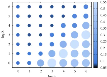
Fig. 2. Error of partitioned gossip learning withS=10 andN=100 on the Pendigits dataset as a function ofη^andλafter 10 cycles (left) and after 1000 cycles (right).

5.4. Hyperparameters

The cycle length parameters ∆g and ∆f were set in two different ways. In thecontinuous transferscenario, the goal was to make sure that the protocols communicate as much as they can under the given bandwidth constraint. The gossip cycle length

∆g is thus exactly the transfer time of a full model, that is, all the nodes send messages continuously. The cycle length ∆f of federated learning is the round-trip time, that is, the sum of the upload and download transfer times. When compression is used, the transfer time is proportionally less as defined by the compression rate, and this is also reflected in the cycle length settings.

In the bursty transfer scenario, we assume that we transfer only during a given percentage of the time, say, 1% of the time. Let δdenote the transfer time and letp∈(0,¹]be the proportion of the time we use for transfer. Here, we set the gossip cycle length

∆g =δ/p. To implement the bursty model in federated learning, we have many choices for the cycle length depending on how many nodes the master wants to contact in a single cycle. If we set∆f =(δup+δdown)/^p(whereδupandδdownare the upload and download transfer times, respectively) then the master should contact all the nodes as before so the only effect is to slow the algorithm down. If we set a shorter cycle length then the master will contact only a subset of the nodes to achieve the required proportion of poverall. We will examine this latter case when the cycle length is set so that 1% of the nodes are contacted in a cycle: ∆f = δup+δdown, where we needp = 1/100 to hold as well. When compression is used,δupandδdownmight differ.

Fig. 3. Error of partitioned gossip learning withS=10 andN=4140 on the Spambase dataset as a function ofη^andλafter 1000 cycles.

In both the bursty and the continuous transfer scenarios, on average, the two algorithms transfer the same number of bits overall in the network during the same amount of time. Further- more, continuous transfer is the special case of bursty transfer withp=1.

As for subsampling, we explore the sampling probability val- uess ∈ {1,⁰.⁵,⁰.²⁵,⁰.¹}. In federated learning, both the up- stream and the downstream messages can be sampled using a

115

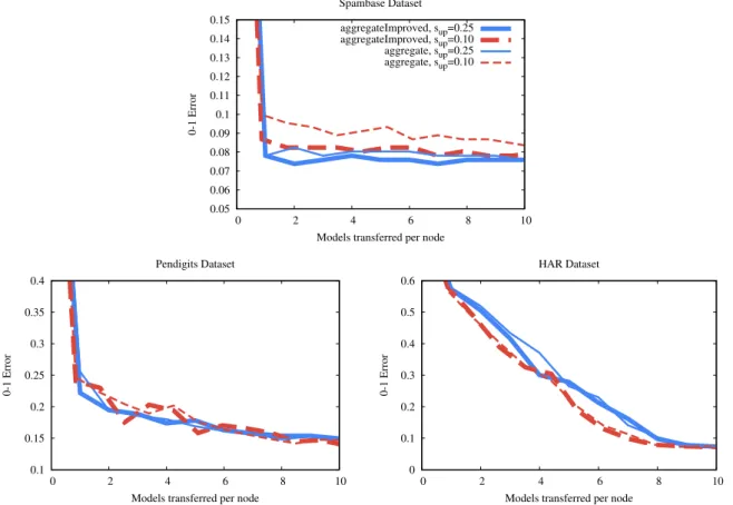
Fig. 4. Federated learning, 100 nodes, long transfer time, no failures, different aggregation algorithms and upstream subsampling probabilities and withsdown=1.

different rate, denoted bys_upands_down, respectively. The setting we use in our experiments is s_down = s_up. However, we shall also show runs where we fix s_down = 1 and experiment with upstream sampling only. When the subsampling is based on partitioning, the number of partitions S defines the sampling probability, which equals 1/S. On the plotss=1/^Swill be used even in the partitioned case to indicate the compression rate.

We train a logistic regression model. For the datasets that have more than two classes (Pendigits, HAR), we embedded the model in a one-vs-all meta-classifier. The learning algorithm was stochastic gradient descent. The learning rate η and the regu- larization coefficient λ used in our experiments are shown in Table 2. We used grid search to optimize these parameters in var- ious scenarios, and found these values relatively robust. However, one should keep in mind that including additional hyperparam- eters in the search, such as the number of iterations (that we simply fixed here), could result in a different outcome.

Although we fixed the parameters shown inTable 2in all the scenarios, it is interesting to have a more fine-grained look at the behavior of these hyperparameters. This sheds some light on possible heuristics to pick the right parameters. All the examples here are measurements with gossip learning without token ac- counts but with model partitioning andS = 10. With network sizeN = 100, over the Pendigits dataset, after 10 gossip cycles, the optimal hyperparameters are η = 10² and λ = 10⁻², as shown in Fig. 2. However, after 100 cycles, the optimal values are η = 10³ and λ = 10⁻³, and after 1000 cycles, η = 10⁴ andλ=10⁻⁴. We often observed similar trends also with other algorithms and datasets. Notice that settings where ηλ = 1 (points on the diagonal of the grid) are often a good choice;

however, there are exceptions. For instance, when we have only one example per node, over the Spambase dataset, this is not the case, as shown inFig. 3. As we can see, here, the points above the diagonal tend to be somewhat better. Also note that settings with ηλ >1 (points below the diagonal) tend to perform very poorly.

Table 2 Hyperparameters.

Spambase Pendigits HAR

Parameterη ^{103 104 102}

Parameterλ ^{10−3 10−4 10−2}

6. Experimental results

We ran the simulations using PeerSim [26]. As for the hard- ware requirements for reproducing our results, we used a server with 8 2 GHz CPUs each with 8 cores, for a total of 64 cores. The server had 512 GB RAM. On this configuration, the experiments we include in this work can be completed within a month.

We measure learning performance with the help of the 0–1 error, which gives the proportion of the misclassified examples in the test set. In the case of gossip learning the loss is defined as the average loss over the online nodes. This means that we compute the 0–1 error of all the local models stored at the nodes over the same test set, and we report the average. In federated learning we evaluate the central model at the master. Note that this is often more optimistic than evaluating the average of the online nodes. For example, in the bursty transfer scenario, or if the downstream communication is compressed (that is,s_down <

1), the local models will always be more outdated than the central one, because the nodes will not receive the complete model, or they receive it with a delay.

The presented measurements are averages of 5 runs with dif- ferent random seeds. The only exceptions are the measurements with our gossip algorithms in the scenarios over the HAR dataset when the network size was the database size. These scenarios are expensive to simulate so we show a single run.

The 0–1 error is measured as a function of the total amount of bits communicated anywhere in the system normalized by

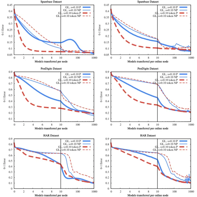
Fig. 5. Gossip learning with one node for each example, bursty transfer, subsampling probabilitys=0.1, no-failure (left) and smartphone trace with long transfer time (right). Variants with and without model partitioning, indicated as P and NP, respectively.

the number of online nodes. We use the size of a full machine learning model as the unit of the transferred information.

6.1. Basic design choices

First, we compare the two aggregation algorithms for sub- sampled models in Algorithm 7 (Fig. 4) in the no-failure con- tinuous transfer scenario. The results indicate a slight advantage ofaggregateImproved, although the performance depends on the database. In the following we will applyaggregateImprovedas our implementation of method_aggregate.

Another design choice is whether we should apply model partitioning. We introduced model partitioning to help token gossip learning. However, this technique has other advantages as well. To verify this, we compared partitioned and non-partitioned variants in several scenarios (Fig. 5). We show the scenario where the effect in question is the clearest. Clearly, the partitioned im- plementations consistently outperform the non-partitioned ones, although in the no-failure scenario, classical gossip learning ap- pears to suffer a temporary setback during convergence. Note that

this is a case where the hyperparameters are not exactly optimal, as we explained in Section5.4,Fig. 3.

The improved performance in the partitioned case is due to the more fine-grained handling of the age parameter. Recall that in the partitioned implementation, all the partitions have their own age and are updated accordingly. In the smartphone trace scenario, this feature is especially useful, since when a node comes back online after an offline period, its model is outdated.

During the first merge operation on the model, only those pa- rameters will get an updated age parameter that were indeed updated, that is, that are included in the merged partition. With- out partitioning, only a random subset of the parameters will be merged, but the entire model will get a new age value. This is a problem because in the first merge operation that they are included in, the weight of these old parameters will be too large.

Due to these observations, from now on, all the experiments are carried out with model partitioning, and this fact will not be explicitly indicated.

The third design choice that we study is the subsampling (that is, compression) strategy for federated learning. Recall that we

117

Fig. 6. Federated learning with 100 nodes, no-failure scenario, with different subsampling strategies ands=0.1. The ‘‘local’’ plot indicates the average of the models that the clients store, otherwise the master’s model is evaluated.

have a choice to subsample only the model that is sent by the client to the master or we can subsample in both directions. Note that if we subsample in both directions then we can achieve a much higher compression rate but the convergence will be slower. Overall, however, it is possible that, as a function of overall bits communicated, it is still preferable to compress in both directions. Note that subsampling only the model from the master to the client is meaningless because that way the client will send mostly outdated parameters that the master has already received in previous rounds.

Fig. 6 compares the two meaningful strategies for the case of s = 0.1. Subsampling in both directions is clearly the better choice. However, it also has a downside, because in that case the clients no longer receive the full model from the master so they cannot use the best possible model locally. To illustrate this problem, we include the average performance of the models stored locally. Depending on the application, this may or may not be a problem. Nevertheless, from now on, we will apply subsampling in both directions in the remaining experiments.

6.2. Continuous transfer

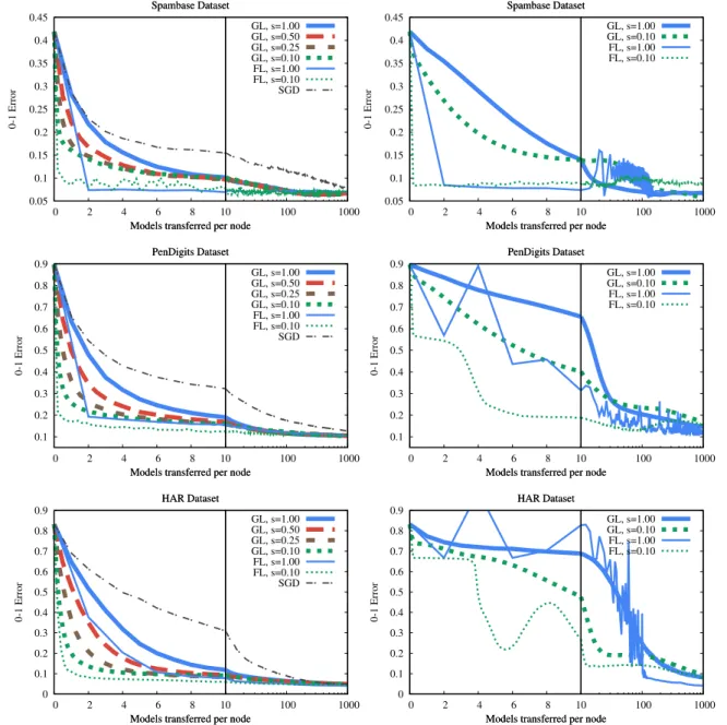
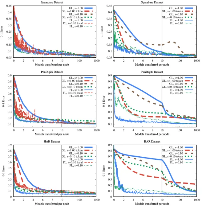
Here, we study the continuous transfer setup where all the nodes try to minimize their idle time taking advantage of the available bandwidth as best as they can. The comparison of the different algorithms and subsampling probabilities is shown in Fig. 7. The stochastic gradient descent (SGD) method is also shown, which was implemented by gossip learning with no merg- ing, where the received model replaces the current model at the nodes. Clearly, the methods using merge are all better than SGD. Also, it is very clear that subsampling helps both federated learning and gossip learning.

Most importantly, in the 100 node setup (left column ofFig. 7), gossip learning is competitive with federated learning in the case

of high compression rates (that is, low sampling probability). This was not expected, as gossip learning is fully decentralized, so the aggregation is clearly delayed compared to federated learning.

Indeed, with no compression, federated learning performs better.

Fig. 7(right) also illustrates the extreme scenario, when each node has only one example, and the size of the network equals the dataset size. This is a much more difficult scenario for both gossip and federated learning. Also, federated learning is expected to perform relatively better, because of the more aggressive cen- tral aggregation of the relatively little local information. Still, gossip learning is in the same ballpark in terms of performance. In terms of long range convergence (recall, that our scenarios cover approximately a day’s time) all the methods achieve good results.

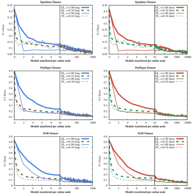
Fig. 8 contains our results over the smartphone trace churn model. Here, all the experiments shown correspond to a period of 24 h, so the horizontal axis has a temporal interpretation as well.

The choice of long or short transfer time causes almost no differ- ence (apart from the fact that the shorter transfer time obviously corresponds to proportionally faster convergence). Also, more interestingly, churn only causes a minor increase in the variance of the 0–1 error but otherwise we have a stable convergence. This is due to the application of model partitioning. Previous results without model partitioning showed a much higher variance. It is also worth pointing out that federated learning and gossip learning shows a practically identical performance under high compression rates. Again, gossip learning is clearly competitive with federated learning.

Fig. 9contains the results of our experiments with the single class assignment scenario, as described in Section 5.1. In this extreme scenario, the advantage of federated learning is more apparent, although on the long run gossip learning also achieves good results. Interestingly, in this case the different compression rates do not have a clear preference order. For example, on the Pendigits database (containing 10 classes) the compressed variant

Fig. 7. Federated learning and gossip learning with 100 nodes (left) and with one node for each sample (right), no-failure scenario, with different subsampling probabilities. Stochastic Gradient Descent (SGD) is implemented by gossip learning with no merging (received model replaces current model).

is inferior, while on HAR (with 6 classes) the compressed variant appears to be preferable.

Let us also point out the similarity between the results on Figs. 9and7(right). Indeed, the scenario where each node has one sample is also a single class assignment scenario by definition.

6.3. Bursty transfer

Here, we study the bursty transfer setup where all the nodes communicate only during a given percentage of the time, as described in Section5.4. Without any modification, the behavior of the algorithms we have discussed so far is very similar to their behavior in the continuous transfer scenario. Although gossip algorithms do work slightly better due to the reduced number of parallel transfers, the bursty transfer scenario offers a possibil- ity to implement specialized techniques that take advantage of bursty transfer explicitly.

In the case of gossip learning, we introduced the token account flow control technique, as described previously. This technique motivated the partition-based sampling technique, to allow for

the formation of ‘‘hot potato’’ chains for each partition separately.

Recall that in Section 6.1 we decided that all the experiments would use model partitioning, after observing that it helps even traditional gossip.

In the case of federated learning, one such technique is when the master communicates only with a subset of the workers in each round, selecting a different subset each time. This way, although the workers communicate in a bursty fashion, the global model still evolves relatively faster. Here, we will assume that the nodes communicate only 1% of the time. In this case, the master will talk to 1% of the nodes in each round. This way, the master communicates continuously while the nodes communicate in bursts.

Fig. 10illustrates the performance in the bursty transfer sce- nario. Clearly, the convergence of each algorithm becomes faster than in the continuous communication case. This suggests that it is better to allow for short but high bandwidth bursts as opposed to long but low bandwidth continuous communication.

We can also observe that token gossip converges faster than

119

Fig. 8. Federated learning and gossip learning over the smartphone trace with long (left) and short (right) transfer time, in the 100 node scenario.

regular gossip in most cases. Also, the best gossip variant is, again, competitive to the federated learning algorithm.

6.4. Large scale

Here, we experiment with the scenario where the number of examples per node was the same as in the 100 node scenario, but the network size equaled the database size. To achieve this, we replicated the examples, that is, each example was assigned to multiple nodes (see Section 5.1). We call this the large scale scenario.

The results are shown in Fig. 11. We can see that the best gossip variants are competitive with the best federated learn- ing variants. The first observation we can make is that in the bursty transfer scenario a faster convergence can be achieved.

This is due to the algorithms that exploit burstiness. Besides, the most important feature of this large scale scenario seems to be whether the label distribution is biased (single label assignment) or not (random assignment). The single class assignment (biased) scenario results in a slower convergence for both approaches.

However, compared with previous experiments, increasing the size of the network in itself does not slow the protocols down.

7. Related work

The literature on machine learning and, in general, optimiza- tion based on decentralized consensus is vast [30]. Our contribu- tion here is a comparison of the efficiency of decentralized and centralized solutions that are based on keeping the data local.

Thus, we focus on works that target the same problem. Savazzi et al. [29] study a number of gossip based decentralized learning methods in the context of industrial IoT applications. They focus on the case where the data distribution is not identical over the nodes. They do not consider compression techniques or other algorithmic enhancements such as token-based flow control.

Hu et al. [17] introduce a segmentation mechanism similar to ours, but their motivation is different. Their focus is on saturating the bandwidth of all the nodes using P2P connections that have a relatively smaller bandwidth, which means they propose that the nodes should communicate to several peers simultaneously.

Fig. 9. Federated learning and gossip learning with 100 nodes, no-failure scenario, with single class assignment.

Sending only a part of the model appears to be beneficial in this scenario. In our case, we focused on convergence speed as a function of overall communication, and we used this technique to optimize our token-based flow control mechanism.

Blot et al. [6] compare a number of aggregation schemes for the decentralized aggregation of gradients, including a gos- sip version based on the weighted push sum communication scheme [20]. Although the authors do not cite federated learning or gossip learning as such, their theoretical analysis and new algorithm variants are relevant and merit further study.

Lalitha et al. [23] study the scenario where each node can possibly observe only a subset of parameters and the task is to learn a Bayesian model collaboratively without a server. The work is mainly theoretical, experimental evaluation is done with two nodes only, as an illustration.

Jameel et al. [18] focus on the communication topology, and attempt to design an optimal topology that is both fast and com- munication efficient. They propose a superpeer topology where superpeers form a ring and they all have a number of ordinary peers connected to them.

Lian et al. [24] and Tang et al. [33] introduce gossip algo- rithms and compare them with the centralized variant. Koloskova et al. [21] improve these algorithms via supporting arbitrary gradient compression. The main contribution in these works is a theoretical analysis of the synchronized implementation. Their assumptions on the network bandwidth are different from ours.

They assume that the server is not unlimited in its bandwidth usage, and they characterize convergence as a function of the number of synchronization epochs. In our study, due to our edge computing motivation, we focus on convergence as a function of system-wide overall communication in various scenarios in- cluding realistic node churn. We perform asynchronous measure- ments along with optimization techniques, such as token-based flow control.

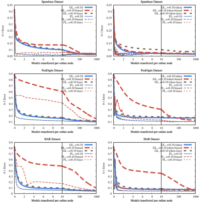
Giaretta and Girdzijauskas [14] present a thorough analysis of the applicability of gossip learning, but without consider- ing federated learning. Their work includes scenarios that we have not discussed here including the effect of topology, and the correlation of communication speed and data distribution.

Ben-Hun and Hoefler [4] very briefly consider gossip alterna- tives claiming that they have performance issues.

8. Conclusions

Here, we compared federated learning and gossip learning to see to what extent doing away with central components—as gossip learning does—hurts performance. The first hurdle was designing the experiments. One has to be careful what system model is selected and what constraints and performance mea- sures are applied. For example, the best algorithm will be very different when we grant a fixed overall communication budget to the system overall but allow for slow execution, or when we give a fixed amount of time and allow for utilizing all the available bandwidth at all the nodes.

Our choice was to allow the nodes to communicate within a configurable bandwidth cap that is uniform over the network, except the master node. This can be done in a continuous fashion, or in a bursty fashion. In the latter case, the cap is interpreted in terms of the average bandwidth usage in any time window of some fixed length. These models cover most application sce- narios. Within these models, we were interested in the speed of convergence after a given amount of overall communication.

We observed several interesting phenomena in our various scenarios. In the random class assignment case (when nodes have a random subset of the learning examples) gossip learning is clearly competitive with federated learning. In the single class assignment scenario, federated learning converges faster, since it can mix information more efficiently. This includes the case

121