The remainder term in Fourier series and its relationship with the Basel problem

(1)

34(2007) pp. 17–28

http://www.ektf.hu/tanszek/matematika/ami

The remainder term in Fourier series and its relationship with the Basel problem

V. Barrera-Figueroa

^a

, A. Lucas-Bravo

^a

, J. López-Bonilla

^b

a Unidad Profesional Interdisciplinaria de Ingeniería y Tecnologías Avanzadas, Departamento de Telemática

e-mail: vbarreraf@ipn.mx, alucasb@ipn.mx

b Instituto Politécnico Nacional, Escuela Superior de Ingeniería Mecánica y Eléctrica, Sección de Estudios de Postgrado e Investigación

e-mail: jlopezb@ipn.mx

Submitted 5 September 2007; Accepted 20 November 2007

Abstract

In this paper it is shown several approximation formulae for the remainder term of the Fourier series for a wide class of functions satisfying specific boundary conditions. Also it is shown that the remainder term is related with the Basel problem and the Riemann zeta function, which can be interpreted as the energy of discrete-time signals; from this point of view, their energy can be calculated with a direct formula instead of an infinite series. The validity of this algorithm is established by means several proofs.

Keywords: Fourier series remainder term, discrete-time signal, Basel problem, slow varying-type series.

1. Introduction

Fourier series is a mathematical tool for characterizing the frequency content of a periodic signal which satisfies the Dirichlet conditions [1]. However, the Fourier series is frequently applied to non-periodic functions, made artificially periodic by extending periodically its original domain. In practice, with a sufficiently large number of terms, a finite expansion can be built upon the Fourier series for repre- senting accurately enough the function. Such finite representation carries implicitly a remainder term which must be estimated [2].

The calculation of the remainder term is expressed via a mean square error between the infinite series and the finite expansion, which provides us an enclosed

17

(2)

range of values where the error can be found, instead of an exact formula. Such estimations stir up the appearance of slow varying-type series, as in the Basel problem series, which in general are expressed by the Riemann zeta function. This let us establish a relation between it and a discrete-time signal, usually defined for all the natural numbers. Therefore the approximation of the remainder term in Fourier series can be employed as an excellent way for calculating the energy of a discrete-time signal. The energy calculation embraces a small number of terms instead of an infinite number, which brings us accurately enough results whose validity is proved in this paper.

2. Integral approach of slow-varying series

In the calculation of the remainder term in finite Fourier expansion, appears series whose members are expressed as the product of a periodic term and a function which varies slowly between successive values of. This let us get a very good approximation of the series [5]:

∞

X

k=1

e^jkαϕ(k). (2.1)

Let us integrate the k^th term aroundk−1/2andk+ 1/2: Z k+1/2

k−1/2

ϕ(ξ)e^jξαdξ = Z 1/2

−1/2

ϕ(k+t)e^j(k+t)αdt

= 1

jαϕ(k+t)e^j(k+t)α

1/2

−1/2

− 1 jα

Z 1/2

−1/2

ϕ^′(k+t)e^j(k+t)αdt. (2.2) However, sinceϕ^′(k+t)tends to zero asymptotically, it is possible to establish the following approximation:

Z 1/2

−1/2

ϕ(k+t)e^j(k+t)αdt≈ e^jkα

jα [ϕ(k+ 1/2)e^jα/2−ϕ(k−1/2)e⁻^jα/2]. (2.3) Because of the slow variation ofϕ(k)we have thatϕ(k+1/2)≈ ϕ(k−1/2)≈ϕ(k), therefore the integral is:

Z 1/2

−1/2

ϕ(k+t)e^j(k+t)αdt≈e^jkαϕ(k)sinα/2

α/2 . (2.4)

By changing the integrating variable we have:

e^jkαϕ(k)≈ α 2 sinα/2

Z k+1/2

k−1/2

ϕ(ξ)e^jξαdξ, (2.5)

(3)

which transforms the original series into a series of integrals:

∞

X

k=1

∞

X

k=1

Z k+1/2

k−1/2

ϕ(ξ)e^jξαdξ. (2.6) Since the integration limits are contiguous, the series becomes in just one integral:

∞

X

k=1

Z ^∞

1/2

ϕ(ξ)e^jξαdξ. (2.7)

3. The Zeta function as the generalization of the Basel problem

The Basel problem is a famous issue in the Number Theory because of its inge- nious solution provided by Leonhard Euler, and its relationship to the distribution of the prime numbers. The problem consists in calculating the exact sum of the following series:

∞

X

n=1

1

n² = lim

n→∞

1 1²+ 1

2²+ 1

3²+· · ·+ 1 n²

. (3.1)

Euler’s method uses the Taylor series for the sine function, which is a polynomial whose roots arex=kπ,k∈Z. Thus, with the Fundamental Theorem of Algebra, the polynomialsinx/xcan be written in terms of its roots [3]:

sinx

x = 1−x² 3! +x⁴

5! +x⁶

7! +· · ·=A(x²−π²)(x²−4π²)(x²−9π²)· · ·, (3.2) whereAis a proportionality constant. Since each factor has the formx²−n²π²= 0, they can be expressed as1−x²/n²π² , transforming the polynomial into:

sinx

x = (1−x²

π²)(1− x²

4π²)(1− x²

9π²)· · ·, (3.3) by multiplying all the factors and gathering the coefficients belonging tox², results the series:

−1 π² − 1

4π² − 1

9π²· · ·=−1 π²

∞

X

n=1

1

n², (3.4)

From (3.2) we get the coefficient of x² as−1/3!, therefore:

∞

X

n=1

1 n² =π²

6 . (3.5)

(4)

The same procedure, after being applied in the other resulting powers of the mul- tiplication (3.3), gives a set of impressive series, all of which are based in even powers:

∞

X

n=1

1 n⁴ =π⁴

90,

∞

X

n=1

1 n⁶ = π⁶

945,

∞

X

n=1

1 n⁸ = π⁸

9450,

∞

X

n=1

1

n¹⁰ = π¹⁰

93555, . . . (3.6) The generalization of the Basel problem for real powers is gotten by the Riemann zeta function, defined as [6]:

ζ(x) =

∞

X

n=1

1

n^x, x6= 1. (3.7)

The case x= 1 is avoided since the series becomes divergent, Figure 1. For even powers the function gives exact values, proportional to even powers ofπ, as shown in (3.6); for odd powers it is not possible to get such an exact representations. The

Figure 1: Plot of the Riemann zeta function.

Bernoulli numbersBn are a set of rational numbers defined by the series [4]:

x e^x−1 =

∞

X

n=0

Bnxⁿ n! , B0= 1, B1=−1

2, B2= 1

6, B4=− 1

30, B6= 1

42, . . . (3.8) The zeta function is related with them for integer values of the argument xas:

ζ(n) = 2ⁿ⁻¹|Bn|πⁿ

n! , Bn= (−1)ⁿ⁺¹nζ(1−n), n∈N. (3.9)

4. The remainder term of Fourier series

The Fourier series develops a function by means of an infinite series of trigono- metric terms; its convergence is assured by Dirichlet conditions. However, in practice, it is not possible to take an infinite number of such orthogonal functions, but a

(5)

finite number of them for performing a finite Fourier expansionfn(x), formed byn terms. Fourier series convergence shows that by taking a sufficiently large number of terms, the difference between f(x)and fn(x), named the remainder term, can be made as small as we desire:

ηn(x) =f(x)−fn(x). (4.1) Let us suppose thatf^(m)(x)exists, although its continuity is not demanded; however, the continuity of f(x), f^′(x), f^′′(x), . . . , f^m⁻¹(x) is required for setting the following boundary conditions:

f(π) =f(−π), f^′(π) =f^′(−π), . . . , f^m⁻¹(π) =f^m⁻¹(−π). (4.2) The existence of the above conditions let us simplify the integration of the coefficients in Fourier series, performed by parts successively m times. They can be gathered in a complex coefficient:

ak+jbk= j^m πk^m

Z π

−π

f^(m)(ξ)e^jkξdξ, (4.3)

where the Fourier series is the real part of the series:

f(x) =

∞

X

k=1

(ak+jbk)e⁻^jkx= Z π

−π

f^(m)(ξ)

"

j^m π

∞

X

k=1

e^jk(ξ⁻^x) k^m

#

dξ. (4.4)

The indexk= 0has been omitted sincef(x)stands forf(x)−a0/2. Let us change the integrating variable by θ= ξ−x, therefore, f(x)is written in terms of the kernel-type seriesGm(θ):

f(x) = Z π

−π

f^(m)(θ+x)Gm(θ)dθ, Gm(θ) = j^m π

∞

X

k=1

e^jkθ

k^m. (4.5) In the finite expansion fn(x), the kernel-type series must add only n terms, thus the remainder term is expressed in function of another kernel-type seriesg_n^m(θ):

ηn(x) = Z π

−π

f^(m)(θ+x)g_n^m(θ)dθ, g_n^m(θ) = j^m π

∞

X

k=n+1

e^jkθ

k^m . (4.6) The simpler method for getting the remainder term is based on Cauchy inequality:

"

Z b

a

f(x)g(x)dx

#2

6 Z b

a

f²(x)dx Z b

a

g²(x)dx. (4.7) After applied it in (4.6) we get:

η_n²(x)6 Z π

−π

f^(m)²(θ+x)dθ Z π

−π

[g^m_n(θ)]²dθ. (4.8)

(6)

In this case, we can take advantage of the orthogonality of the members of the series g_n^m(θ), by taking their real part. The integral of the square of kernel-type series is:

Z π

−π

[g_n^m(θ)]²dθ= 1 π²

∞

X

k=n+1

Z π

−π

coskθ k^m

∞

X

l=n+1

coslθ l^m dθ= 1

π

∞

X

k=n+1

1

k^2m. (4.9) The above series seems to be related with the Riemann zeta function, however, we cannot get an exact result since the series starts from n+ 1. For estimation purposes, we can use the integral approach of a slow varying-type series, whose periodic part is the unitary function, i.e., α = 0. The slow varying part is the function ϕ(k) = 1/k^2m, which varies slowly, since m and n are supposed to be great:

1 π

∞

X

k=n+1

1 k^2m ≈ 1

π Z ^∞

n+1/2

dξ

ξ^2m = 1

π(2m−1)(n+ 1/2)^2m⁻¹. (4.10) The integral of f^(m)², should be identified as the norm of the m^th derivative of f(x), represented by N_m², therefore the remainder term is bounded by:

|ηn(x)|< Nm

pπ(2m−1)(n+ 1/2)^m⁻^1/2. (4.11) Another method for getting the remainder term is by evaluating reliably the kernel- type series g^m_n(θ)with the integral approach of a slow varying-type series, where the slow varying function corresponds with ϕ(k) = 1/k^m. With the exception of small values aroundθ= 0, we can use the asymptotic behavior of the integral:

g_n^m(θ)≈ j^mθ 2πsinθ/2

Z ^∞

n+1/2

e^jξθ

ξ^mdξ≈ j^m+1 2πsinθ/2

e^j(n+1/2)θ

(n+ 1/2)^m. (4.12) For estimation purposes, the remainder term can be calculated by means the following inequality:

|ηn(x)|6 Z π

−π

|f^(m)(θ+x)||g_n^m(θ)|dθ=|f^(m)(x)|max

Z π

−π

|g^m_n(θ)|dθ. (4.13) After taking the real part ofg_n^m(θ)and integrating it, we get the following formula:

|ηn(x)|< 2 (n+ 1/2)^m⁻¹

ln(n+ 1/2)π

(n+ 1/2)π |f^m(x)|max. (4.14)

5. Mean square error in Fourier series

Frequently the remainder term is known as the error term, for its interpretation is obvious. However, it is more suitable to handle a mean square error for practical issues:

η²= 1 2π

Z π

−π

η²_n(x)dx= 1 2π

Z π

−π

[f(x)−fn(x)]²dx. (5.1)

(7)

The orthogonality properties let us express the mean square error in function of the coefficients in Fourier series:

η²=1 2

∞

X

k=1

(a²_k+b²_k)−1 2

n

X

k=1

(a²_k+b²_k) =1 2

∞

X

k=n+1

(a²_k+b²_k), (5.2) where the mean square error results equal to the square of the remainder term:

η²= η²_n 2π

Z π

−π

dx=η²_n. (5.3)

The above formulae let us find out a relation between the norm of them^thderivative off(x)and the coefficients of its Fourier series. By substituting (4.9) into (4.8) we have:

η_n² 6 1 π

∞

X

k=n+1

1 k^2m

Z π

−π

f^(m)²(ξ)dξ, (5.4)

from which we get the following inequality:

1 2

∞

X

k=n+1

(a²_k+b²_k)6 1 π

∞

X

k=n+1

1 k^2m

Z π

−π

f^(m)²(ξ)dξ, (5.5) which provides us the wanted relation:

a²_k+b²_k < 1 πk^2m

Z π

−π

f^(m)²(ξ)dξ. (5.6)

If we consider that in the inequality (5.5) both series start from k= 1, we get:

1 2

∞

X

k=1

(a²_k+b²_k)6 1 π

∞

X

k=1

1 k^2m

Z π

−π

f^(m)²(ξ)dξ, (5.7) where the left side is proportional to the integral of f²(x):

∞

X

k=1

(a²_k+b²_k) = 1 π

Z π

−π

f²(x)dx, (5.8)

from which the following inequality is gotten:

1 2

Z π

−π

f²(x)dx6

∞

X

k=1

1 k^2m

Z π

−π

f^(m)²(ξ)dξ. (5.9) This series is expressed in terms of the zeta function, from which results the following impressive inequality:

Z π

−π

f²(x)dx6 (2π)^2m (2m)! |B2m|

Z π

−π

f^(m)²(ξ)dξ. (5.10)

(8)

6. Energy of discrete-time signals

A discrete-time signalx(k)is a single value function defined at discrete points of the domain, which represents the samples of a continuous-time function xa(t), related with the first one by:

x(k) =xa(kT), k∈Z, (6.1) being T the sampling rate. For discrete-time signals we can define their energyE as that dissipated by a unitary resistance:

E=

∞

X

k=−∞

|x(k)|². (6.2)

For energy signals, the above series converges. However, if the series diverges, the function is said to be a power signal [7]. In general, power signals are periodic functions, where their mean powerP, measured in a complete periodN, converges:

P= lim

N→∞

1 2N+ 1

N

X

k=−N

|x(k)|². (6.3)

In practice, it is not possible to perform an infinite summation for calculating the energy of a discrete-time signal, since with a representative number of terms we can get an approximation of the series, for the upper terms can be neglected since energy signals show a decreasing behavior; therefore we have the following approximation:

En=

n

X

k=1

|x(k)|², (6.4)

where x(k)is supposed to be a causal signal, i.e., x(k) = 0 fork 60. Therefore, the Riemann zeta function, for even arguments, gives the exact value of the energy of a discrete-time signal:

E=ζ(2m) =

∞

X

k=1

1

k^2m, m∈N. (6.5)

which is written as a sequence of weighted unitary impulse:

x(n) =

∞

X

k=1

δ(n−k)

k^m , δ(n−k) =

1, n=k,

0, n6=k. (6.6)

The approximation of the energy of the signal is written in terms of its total energy, expressed by the zeta function:

En=

n

X

k=1

1

k^2m =ζ(2m)−

∞

X

k=n+1

1

k^2m. (6.7)

(9)

In this formula, we can use the integral approach of a slow varying-type series since the second one varies slowly, as is required. Therefore:

∞

X

k=n+1

1 k^2m ≈

Z ^∞

n+1/2

dξ

ξ^2m = 1 (2m−1)

1

(n+ 1/2)^2m⁻¹. (6.8) Hence, the next formula has the advantage of bring us a very accurate value of the energy of the discrete-time signal without developing the sum until then^th term:

En≈ζ(2m)− 1 (2m−1)

1

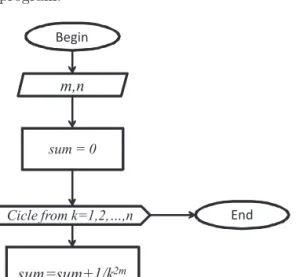
(n+ 1/2)^2m⁻¹. (6.9) The following tables present a comparative analysis which demonstrates the validity of (6.9) as a reliable approximation formula for the finite expansion (6.4). For doing so, we must programming the formula (6.7) by using double precision floating point variables, defined in C++ language like of double type. Figure 2 shows the flow diagram of the main program.

m,n

sum = 0

Cicle from k=1,2,…,n Begin

End

sum=sum+1/k^2m

Figure 2: Algorithm for performing the expansionEn.

7. Conclusions

The formulae used for getting the bounded values of the remainder terms were deduce from the integral approach of a slow varying-type series, which let us cal- culate the remainder term without performing the infinite sum of the series. In fact, in this work has been proved that the remainder term can be related with the Riemann zeta function, which aroused from the Basel problem.

(10)

n En En Absolute

summation approximation Difference

1 1.000000000000000000 0.978267400181559776 0.021732599818440224 10 1.549767731166540760 1.549695971610131060 0.000071759556409701 100 1.634983900184892260 1.634983818092007550 0.000000082092884712 1000 1.643934566681561240 1.643934566598351350 0.000000000083209883 10000 1.644834071848064960 1.644834071847976360 0.000000000000088596 100000 1.644924066898243000 1.644924066898226120 0.000000000000016875

Table 1: Casem= 1.

n En En Absolute

1 1.000000000000000000 0.983557801612372495 0.016442198387627505 10 1.082036583493756640 1.082035287844960840 0.000001295648795807 100 1.082322905344472730 1.082322905328218180 0.000000000016254553 1000 1.082323233378305940 1.082323233378304160 0.000000000000001776 10000 1.082323233710861480 1.082323233710804630 0.000000000000056843 100000 1.082323233710861480 1.082323233711137480 0.000000000000276001

Table 2: Casem= 2.

n E_n E_n Absolute

1 1.000000000000000000 0.991005613424777998 0.008994386575222002 10 1.017341512441431340 1.017341494932115790 0.000000017509315553 100 1.017343061964943730 1.017343061964941290 0.000000000000002442 1000 1.017343061984441020 1.017343061984448570 0.000000000000007550 10000 1.017343061984441020 1.017343061984448790 0.000000000000007772 100000 1.017343061984441020 1.017343061984448790 0.000000000000007772

Table 3: Casem= 3.

The Riemann zeta function can be parsed as the energy of a discrete-time energy signal. For calculating accurately its total energy, it is not necessary to perform a large expansion of terms, but to use a formula which is gotten from the study of the remainder term of the Fourier series.

As can be seen from Tables 1– 5, the results demonstrate the virtue of using the formula (6.9) instead of countingnterms. Even if the expansion is formed by only one term, the error involved is in the order of0.1%form= 5, and2.1%form= 1.

In addition, from the tables we can assure the convergence of the results by taking only ten terms in all of the cases; by taking a large number of terms, the results show that occur a kind of saturation in the results of the program, since there

(11)

n En En Absolute

1 1.000000000000000000 0.995716261417096016 0.004283738582903984 10 1.004077346255262570 1.004077346045353590 0.000000000209908979 100 1.004077356197943030 1.004077356197942580 0.000000000000000444 1000 1.004077356197943030 1.004077356197943920 0.000000000000000888 10000 1.004077356197943030 1.004077356197943920 0.000000000000000888 100000 1.004077356197943030 1.004077356197943920 0.000000000000000888

Table 4: Casem= 4.

n E_n E_n Absolute

1 1.000000000000000000 0.998104320141845691 0.001895679858154309 10 1.000994575058549610 1.000994575056194600 0.000000000002355005 100 1.000994575127818200 1.000994575127817750 0.000000000000000444 1000 1.000994575127818200 1.000994575127817750 0.000000000000000444 10000 1.000994575127818200 1.000994575127817750 0.000000000000000444 100000 1.000994575127818200 1.000994575127817750 0.000000000000000444

Table 5: Casem= 5.

exist no variations in the calculations while increasing the number of summands.

This can be interpreted as that the first elements have more energy than the upper ones. Therefore, the use of a finite expansion for calculating the energy of the discrete-time signal is justified, since the upper terms can be neglected.

References

[1] Cantor, G., Contributions to the Founding of the Theory of Transfinite Numbers Dover Publications, Inc.(1995), 1–82.

[2] Fejér, L., Untersuchen Über Fouriersche Reihen, Math. Annalen, Vol. 58 (1904), 51–69.

[3] Kimble, G., Euler’s Other Proof,Mathematics Magazine, Vol. 60 (1987), 282.

[4] Lanczos, C., Discourse on Fourier Series,Oliver & Boyd, Edinburgh, (1996), 45–75, 109.

[5] Lanczos, C., Linear Differential Operators,Dover Publications, Inc.(1997), 49–99.

[6] Penrose, R., The Road to Reality,Jonathan Cape, (2004), 211.

[7] Proakis, J.G., Manolakis, D.G., Digital Signal Processing. Principles, Algorithms and Applications,Prentice Hall (1999), 43–52.

(12)

V. Barrera-Figueroa and A. Lucas-Bravo

Av. I.P.N. No. 2580 Col. Barrio La Laguna Ticomán, CP 07340, México D.F.

J. López-Bonilla

UPALM Edif. Z-4, 3er piso, Col. Lindavista CP 07738, México D.F.