Real-Time Estimation of Emissions Emerging from Motorways Based on Macroscopic Traffic Data

Real-Time Estimation of Emissions Emerging from Motorways Based on Macroscopic Traffic Data

Alfréd Csikós

, István Varga

a Budapest University of Technology and Economics, Department of Control and Transport Automation, Bertalan Lajos utca 2, H-1111 Budapest, Hungary e-mail: csikos.alfred@mail.bme.hu

b Systems and Control Laboratory, Computer and Automation Research Institute, Hungarian Academy of Sciences, Kende u. 13-17, H-1111 Budapest, Hungary

Abstract: In this paper a complex traffic emission modeling approach is suggested: based on the considerations of macroscopic traffic flow modeling and an average speed emission model, a macroscopic emission model is formed. The proposed methodology leads to two functions to evaluate traffic emission: a model for actually realized emissions and one for the emission level of traffic. The former one is useful for a more exact estimation of emissions relative to inventory methods; the latter one is for the analysis of optimal traffic control objectives. The introduced functions are validated in VISSIM/MatLab environment on a real motorway segment model located in Hungary.

Keywords: traffic emission modeling; macroscopic traffic modeling; freeway traffic flow

1 Introduction

Sustainable development, a catchword of modern times is more relevant than ever.

Road traffic provides a variety of fields in which the ideas of sustainable development challenge engineers. As mobility needs of developed countries increase permanently, several issues arise: delays caused by congestions directly effect national economic performance, while excessive fuel consumption aggravates the exhaustion of wastable energy sources and emissions are responsible for global (greenhouse effect) and local damage (air pollution leading to health issues, acid rain, etc). While traffic control strategies have been widely used to moderate delays and prevent traffic congestion, emission and fuel consumption optimization have only entered the limelight in the relatively recent past. The overlapping of the optima of travel times and emission is not straightforward. In order to formulate control objectives for emission optimization, an understanding of the nature of traffic emission is essential. The current paper

aims to achieve this goal via an analytic traffic emission model that uses real time loop detector measurements.

of road traffic in terms of emissions have been analysed by a variety of models and methods. To estimate the evolved emissions on public roads, emission inventories have been carried out using different emission models such as COPERT and Versit+ [1], [12]. The idea expanded to urban networks in [6]. A more sophisticated approach towards emission estimation is introduced in [12]

using speed measurements of loop detectors for inventories. However, other traffic variables such as traffic density have not yet been utilized during emission estimation and total emission is based on total vehicle miles travelled only; no real-time emission level is considered. The idea of real-time data use is mentioned in [8] but used only on microscopic level for the evaluation of macroscopic control measures (speed limits). Emission modeling for traffic control purposes has been used [15], [18] – but though these models are based on reasonable theoretic considerations, they have not yet been validated.

In our research, a long-term perspective is to design a control method on freeway traffic that minimizes traffic emission as well as travel times. The main idea of our approach is that the emerging traffic demand must be serviced by an infrastructure having a capacity limit lower than the demand level. This capacity defect leads to a low system performance or, in worst case, congestion. Traffic performance in the conventional manner means travel times, but another performance criterion can be the amount and composition of emitted pollutants. The idea of using real- time macroscopic traffic data presents itself during emission modeling.

The paper presents a complex traffic-emission model. It serves dual purposes: on the one hand, the emission optimum of the traffic is sought; on the other hand, total emission of freeway traffic as a function of real-time traffic data may serve as a more exact approach to emission estimation.

The model is introduced on freeway traffic as motorways turn over a significant transport performance, and loop detector measurements provide fairly exact information on traffic conditions. High emission levels are typical of motorways because of the speed range. In addition, the lack of frequent stops and the range of freeway travelling speeds mean that acceleration can be neglected [3], [4] which justifies the use of average speed models.

The suggested model is presented in four sections. After the introductory section, preliminaries regarding freeway traffic models and emission modeling are summarized. The following section proposes a complex modeling approach for traffic emission. Finally, in Section 0, a simulation is carried out on an existing motorway stretch near Budapest for model validation.

2 Preliminaries

2.1 Macroscopic Freeway Traffic Modeling

Freeway traffic is most commonly described with macroscopic traffic models.

This approach considers traffic as compressible fluid, neglecting individual vehicle dynamics, describing it by aggregated variables such as traffic flow – denoted by q [veh/h], traffic density – denoted by ρ [veh/km] and space mean speed – denoted by v [km/h] of traffic. The model was originally derived in continuous-time, whereas the aforementioned variables can only be measured in discrete temporal and spatial intervals. Thus, a temporally and spatially discretized description was formed. First order models characterize flow speed as a static function of traffic density (2), whereas second-order modeling [10] engages a speed momentum equation (3) in addition to the equilibrium relation (2) of traffic mean speed and density. In the proposed complex model, second order modeling is considered.

The equations of the second-order model regarding segment i at discrete time step k are as follows:





) ( ) 1

( q ₁ k q k r k s k

L k T

k _{i i i i}

i i

i    _   

 ⁽¹⁾















 



 





a

cr i free

i

i v a

V 

 ) exp ¹ 

( (2)

 

   



















 

 

 



 



 





















) (

) ( ) ( )

(

) ( ) (

) ( ) ( ) ( )

( ) ( )

( ) 1 (

1

1

k k v k r L

T k

k k L T

k v k v k L v k T v k T V k v k v

i i i i

i i

i i

i i

i i

i (3)

) ( ) ( )

(k k v k

q_i _i  _i ⁽⁴⁾

where q_i, ρi and v_i denote respectively the flow, traffic density and mean speed of segment i, r_i denotes the flow of an on-ramp, s_i the flow of an off-ramp of segment i, while a, β, ρcr, κ, τ, δ, vfree, and η are additional constant parameters [9].

2.2 Emission Modeling Based on Copert Model

During our analysis the utilized model is COPERT IV for hot running emissions.

The model has been extensively used for road traffic emission modeling [2], [17].

COPERT is an average speed model, i.e. emission factors of different pollutants [g/km] are m-order polynomial functions of the average speed devised by certain driving profiles. For vehicle j and pollutant p, see (5). As average speed contains driving pattern data [13], the sole model input variable is average speed. The

emission factor functions are specific for different vehicle classes, fuel types, Euro norms and engine capacities.

] / [ ...

) ( )

( )

(t v t ₁v ¹ t ₀ g km

ef_j^p _m^p _j^m _m^p_{ j}^m  ^p

(5)

Emission factors are most useful in the case of emission inventories: inventories calculate total traffic emission, denoted as te [g] using the following formula (EEA Technical report): te= al∙ef, where ef denotes the emission factor, al is the activity level – the number of vehicles that completed a certain distance on a roadway [vehkm] (abbreviated as VKT – total vehicle kilometers travelled). These data can be obtained by offline data of traffic surveys, considering O-D demands and assignment information, or loop detector measurements. In our case, a different approach is carried out, as total emission is calculated by using emission rates [g/h] and integrated by temporal and spatial variables. The relationship between emission rate e_j^p and emission factor ef_j^p of vehicle j for pollutant p is straightforward [14]:

) ( ) ( )

(t ef t v t

e^p_j  _j^p  _j

(6)

where v_j(t) denotes the instantaneous speed of vehicle j. The formula can be generalized for average emission factors and average emission rates for time intervals if instantaneous speed is substituted by trip-based average speed.

Remark on notations: for the aggregated emission factors of the whole traffic on a segment the appellation of emission level [vehg/km], for aggregated emissions rates of the whole traffic on a segment during a discrete sample step the title total emission rate [vehg/sample step] is used.

3 Methodology

In this section the macroscopic modeling method is introduced using the macroscopic description of traffic and average speed emission modeling.

Consider a homogeneous platoon of vehicles (identical vehicle class and engine type). The assumption is only for the sake of notation simplicity, further on heterogeneous traffic is considered as well (in this case coefficients αi p are the same for all vehicles). Emission rate for vehicle j of pollutant p:

] / [ ) ( ...

) ( )

( )

(t v ¹ t ₁v t ₀v t g h

e^p_j 







(7)

For a vehicle count of N:

] / [ ) ( ...

) ( )

( )

( )

(

1

0 1

1 1

, t v t v t v t vehg h

e t E

N

j

j m p

j p m m

j p m N

j t p j

p 





 









 ⁽⁸⁾

Divide the motorway on segments of number n (spatial discretization). L_i denotes the length of segment i, i,j denotes vehicle number j on segment number i. A total of N_i vehicles are present on segment i. Note that N_i=N_i(t), thus the number of vehicles on segment i is a function of time.

] / [ )) ( ...

) ( )

( (

) (

1 1

, 0 ,

1 1

, t v t v t vehg h

v t

E

n

i N

j

j i m

j i m m

j i m

p 



  

  

 ⁽⁹⁾

On segment i:

] / [ )) ( ...

) ( )

( (

) (

1

, 0 ,

1 1

, t v t v t vehg h

v t

E

Ni

j

j i m p

j i p m m

j i p m p

i 



      ⁽¹⁰⁾

Assuming that each vehicle dwelling in the same segment is travelling with the same speed:

] / [ )) ( ...

) ( )

( (

) ( )

(t N t v ¹ t ₁v t ₀v t vehg h

E_i^p  _i _m^p _i^m _m^p_{ i}^m  ^p _i 

(11)

Remember, that N_i=N_i(t), which is also N_i(t)=ρi(t)L_i

] / [ )) ( ...

) ( )

( (

) ( )

(t t L v ¹ t ₁v t ₀v t vehg h

E_i^p _{i i} _m^p _i^m _m^p_{ i}^m  ^p _i 

(12)

For the sake of simplicity, convert emission rate to a dimension of [veh g/s]:

] / [ )) ( ...

) ( )

( ( ) 3600 ( ) 1

(t t L v ¹t ₁v t ₀v t vehg s

E_i^p  _{i i} _m^p _i^m _m^p_{ i}^m  ^p _i  ⁽¹³⁾ Consider (13) with temporally discrete variables – on segment i, speed of each i,j vehicle is approximated with the mean speed of segment i; ρi(k) is available from loop detector measurements/calculated using the fundamental equation of macroscopic traffic flow (4): T_S denotes sample time.

] /

[

)) ( ...

) ( )

( ( ) 3600 ( )

( ¹ _{1 0}

step sample g

veh

k v k

v k

v L T k

k

E_i^{p S} _{i i m}^p _i^m _m^p _i^{m p} _i









   ^  _ 

(14)

Equation (14) proposes a formula of the emission of traffic emerging on segment i at time step k. The summation by time steps equals to the estimation of the pollution emerged on segment i during the analysed time interval. The summation by length (segments) leads to the emission of the analysed motorway stretch in sample step k (15).

] /

[

)) ( ...

) ( )

( ( ) 3600 (

) (

1

0 1

1

step sample g

veh

k v k

v k v L T k

t E

n

i

i m p

i p m m

i p m i i p S













 

  





(15)

The relationship between emission rate and emission factor is discussed in Section 2.2. In this case, the speed variable of emission factor is the average speed of segment i at time step k.

Thus, using (12), emission level (aggregated emission factors) of segment i at time step k:

] / [ ) ...

) ( )

( ( ) ( )

(k k L v k ₁v ¹ k ₀ vehg km

EF_i^p _{i i} _m^p _i^m _m^p_{ i}^m  ^p 

(16)

The point of the formula is straightforward: traffic emission level is obtained by the real-time summation of individual vehicle’s emission factors in a spatially and temporally discrete manner.

In case of inhomogeneous traffic composition, the formulas are as in (16) and (17). As single-variable polynomials of order m (in this case the emission factors) constitute an m-dimensional linear space, the total emission rate and emission level functions turn out as linear combinations of total emission rates and levels of traffic fractions containing different vehicle types:

] /

[ ) ( ) ( )

(

1

, k vehg samplestep E

k k

E

c c N

c

c p i p

i 





 ⁽¹⁷⁾

] / [ ) ( ) ( )

(

1

, k vehg km

EF k k

EF

c c

N

c

c p i p

i 





 ⁽¹⁸⁾

In equations (17) and (18) c denotes vehicle type, N_c denotes the number of vehicle types, γc denotes the proportion of vehicle class c of whole traffic.

Remark 1: equations (14) and (16) show that real emission and emission levels are both modular – containing emission factors and macroscopic variables. The emission factors can be framed with functions from other average speed emission models. This establishment means a further analysis in future – the comparison of emission models for real-time emission estimation based on macroscopic traffic data.

Remark 2: the emission inventory-based approach (introduced in [12]) can be considered an exaggerated real time emission function – using only one loop detector for a long road stretch.

Remark 3: emission level functions of different pollutants are also applicable as route costs of transportation assignment problems [11], thus taking fuel consumption and environmental impact into account during process design.

0 10 20 30 40 50 60 70 0

50 100

0 50 100 150 200

Traffic density [veh/km]

Traffic speed [km/h]

CO total emission rate [veh g/sample step]

Figure 1

Total emission rate of CO on a 1 km long motorway stretch

0 10 20 30 40 50 60 70

0 50

100 0 100 200 300 400 500 600

Traffic density [veh/km]

Traffic speed [km/h]

CO emission level [veh g/km]

Figure 2

Emission level of CO on a 1 km long motorway stretch

The total emission rate and emission level functions of CO are illustrated in Figs.

1 and 2, using (17) and (18) for a 1 km long motorway stretch, considering the static fleet composition of Hungary from year 2010 (see Table 2) The plot of emission level (Fig. 2) clearly shows that for any traffic density, extremum can be reached by an optimal velocity independent of density, which provides the minimum of the emission factor function – in case of second order traffic modeling. Substituting (2) to (16), a single-variable function arises for the case of first order modeling. (For model parameters of (2) a least-squares fitting of real loop detector measurements of motorway M5 (see Section 0) was carried out.) The function is shown as a curve on the 3D plots. Remember section 2.1- first order traffic modeling means a static relationship between traffic density and traffic speed, while real traffic states and measurements may differ from this curve, and are plotted as dots on both Figs. 1 and 2. The idea of using first order traffic modeling, or at least reducing the range of possible density-speed combinations is another possible research area.

4 Validation

4.1 Simulation Setup

The proposed models were validated on an existing motorway stretch at the border of Budapest: on the M5 motorway from waymark 15 km to 28 km, in both directions. A 30 minute-long period was simulated using VISSIM, and the data were evaluated using MatLab. VISSIM is a microscopic traffic simulation software that is capable of performing loop detector measurements. For the software setup see Fig. 3.

Figure 3

Software environment for model validation

The validation of the macroscopic models was executed in the following way:

emission rates and emission factors of each individual vehicle were modeled and aggregated spatially and temporally by segments and time steps. During the microscopic simulation, simulation step was 1 sec, and the average speed model was utilized in a quasi continuous manner, assuming that average speed of each simulation step is the instantaneous speed at that certain moment. This was considered as the reference or real emission of traffic participants (microscopic modeling). At the same time, loop detector measurements were carried out and utilized as discussed in Section 0 (macroscopic modeling). Loop detector measurements are assumed to offer classified average speeds by vehicle classes.

Both functions introduced in the previous section (emission levels and total emission rates) were compared to reference emissions. Using the model equations, the following pollutants were analysed: CO₂, CO, HC (VOC), NO_X.

Macroscopic traffic measurements can be realized in a temporally and spatially discrete manner. Measurement sample step size was 10 sec so that the Courant–

Friedrichs–Lewy condition is satisfied (i.e. no particle (in this case vehicle) can skip a spatial step during a temporal step). Different loop detector (LD) distances were tested and compared (500 m, 1000 m, 5000 m and an extreme case – only one loop detector in each direction). This was carried out by evaluating only the designated loop detectors. For the loop detector layout see Fig. 5. The evaluated LD measurements for different LD distance cases are summarized in Table 1.

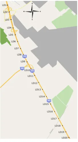
Figure 4

Location of motorway stretch

Figure 5 Loop detector (LD) layout

Table 1

Evaluated loop detector measurements LD distance Evaluated LD no.

500 m all

1000 m 1, 3, 5, 7, 9, 11, 13, 15, 17, 19

5000 m 5, 15

13000 m 9

In the simulations heterogeneous traffic was generated. This heterogeneity was modeled based on the Hungarian static fleet composition of year 2010, the composition of which contains as many as 35 different vehicle classes. In our study, the most frequent vehicle types of each significant vehicle class were considered; this reduced fleet composition made 64.84% of Hungarian static fleet composition of that certain year. For the considered vehicle types see Table 2.

Table 2

Fleet composition of simulation Vehicle

category

Engine type, Euro norm Fraction [%]

Normed fraction for simulation [%]

PC

Gasoline, Euro1, 1.4-2.0l 12.46 19.22 Gasoline, Euro3 1.4-2.0l 12.46 19.22 Diesel, Euro1 <2.0l 9.78 15.08 Diesel, Euro3 <2.0l 10.13 15.62

LDV (<3.5 t)

Diesel, Euro1 2.91 4.49

Diesel, Euro2 1.73 2.67

Diesel, Euro3 2.00 3.08

HDV (Rigid, <7.5 t)

Diesel, Euro1 5.86 9.04

Diesel, Euro2 3.49 5.38

Diesel, Euro3 4.02 6.20

Total 64.84 100

During the simulation, different traffic states were generated: free flow conditions (low traffic flow volumes, high traffic speeds), saturated flow (high traffic flow volumes, near critical density), and congested situations (above critical density, and high density situations); these three rather differing situations are the most characteristic and significant states concerning traffic. For the first 15 minutes, free flow and saturating traffic conditions were simulated. From the 16^th minute, an accident and then a subsequent 10 minute-interval of slow progression was modeled (from 15 min to 25 min). The transitions among traffic states were realized in all directions (congesting and yielding traffic).

The simulated accident occurs at segment no. 13, north-south direction and since motorway accidents usually lead to bottlenecks, significant changes in traffic density, speed and also in emission can be observed. Therefore, total emission rates and emission levels are illustrated on this particular segment (Figs. 6 and 7).

Until the 100^th step (1000 sec) free flow traffic is present with no congestion. The accident happens at 1000 sec, and leads to a solid increase in traffic density until 1200 sec, when the congestion is formed. The congestion starts to dissolve at 1600 sec, and the density on segment no 13 starts decreasing.

4.2 Evaluation of Results

This extreme traffic situation is suitable for comparing the accuracy of different LD configurations, measurement points deployed at different distances. Both total emission rates and emission levels are most accurate estimations of reference emission if loop detectors are at 500 m distances, and accuracy declines with increasing loop detector distance. Emission level estimations (Fig. 8) show that a rare ordination of loop detectors leads to delayed measurement of the extreme

traffic state as the effect appears at distant measurement points with delays. For control design purposes, the most dense loop detector layout is advised because the density of loop detectors along a roadway is in direct proportion to the spatial and temporal accuracy of emission levels. In case of distant loop detectors, application of state estimation is advised which has been successfully utilized for traffic variables [16].

40 60 80 100 120 140 160 180

0 5 10 15 20

CO

Segment no. 13 - total emission rates [veh g/sample step]

40 60 80 100 120 140 160 180

0 0.2 0.4 0.6 0.8

HC

40 60 80 100 120 140 160 180

0 5 NOX

Macroscopic model - LD distance 500m Macroscopic model - LD distance 1000m Macroscopic model - LD distance 5000m Macroscopic model - LD distance 13000m Microscopic model

40 60 80 100 120 140 160 180

0 50 100 150

Sample step [10s]

Traffic density [veh/km/lane]

Figure 6

Traffic density, and total CO and HC emission rates of segment 13, north-south direction

40 60 80 100 120 140 160 180

0 10 20

CO

Segment no. 13 - total emission rates [veh g/sample step]

40 60 80 100 120 140 160 180

0 500 1000 1500

CO2

40 60 80 100 120 140 160 180

0 2 4 6

NOX

Macroscopic model - LD distance 500m Macroscopic model - LD distance 1000m Macroscopic model - LD distance 5000m Macroscopic model - LD distance 13000m Microscopic model

40 60 80 100 120 140 160 180

0 50 100 150

Sample step [10s]

Traffic density [veh/km/lane]

Figure 7

Total CO2 and NOX emission rates of segment 13, north-south direction

40 60 80 100 120 140 160 180 0

100 200 300

CO

Segment no. 13 - emission levels [veh g/sample step]

40 60 80 100 120 140 160 180

0 5 10 15

HC

40 60 80 100 120 140 160 180

0 1 2x 10⁴

CO2

40 60 80 100 120 140 160 180

0 50 100

NOX

Sample step [10s]

Macroscopic model - LD distance 500m Macroscopic model - LD distance 1000m Macroscopic model - LD distance 5000m Macroscopic model - LD distance 13000m Microscopic model

Figure 8

Emission levels of segment 13, north-south direction

Numerical results of simulation for the whole motorway stretch are summarized in Tables 3 to 6, where averages of absolute relative errors (calculated for each discrete step) referred to microscopic modeling are displayed. The most interesting observation of figures is that dense loop detector measurements offer a reasonable estimation of emissions; however, the case of one detector only (LD distance 13000 m) which can be considered as classic inventory calculation may lead to more than 80% of relative errors of real emissions in extreme or changing traffic conditions and relative error is considerable even under free flow conditions (south-north direction). Thus, when consideringusing real-time data, as many loop detectors is advised for a more accurate emission estimation.

Table 3

Average absolute relative differences of total emission – relative to microscopic modeling North-south direction South-north direction

LD distance [m] 500 1000 5000 13000 500 1000 5000 13000

Pollutant

CO 0.1314 0.2332 0.3635 0.5776 0.1137 0.1182 0.2510 0.3230 HC 0.1128 0.1439 0.4119 0.6850 0.1223 0.1510 0.2352 0.4674 CO2 0.0790 0.1094 0.4817 0.8176 0.0868 0.1123 0.3465 0.3952 NO_X 0.1188 0.1529 0.4246 0.5762 0.1304 0.1543 0.2868 0.2707

Table 4

Average absolute relative differences of emission level – relative to micsroscopic modeling North-south direction South-north direction

LD distance [m] 500 1000 5000 13000 500 1000 5000 13000

Pollutant

CO 0.1762 0.1960 0.4222 0.6728 0.1509 0.1607 0.1981 0.3280 HC 0.0714 0.1764 0.3280 0.5821 0.0789 0.0790 0.1805 0.4084 CO2 0.0331 0.1397 0.2933 0.7604 0.0401 0.0595 0.2983 0.5629 NO_X 0.0436 0.1519 0.2546 0.5371 0.0518 0.0819 0.1466 0.3093

Table 5

Average absolute relative differences of total emission – segment 13, north-south direction Segment 13, north-south direction

LD distance [m] 500 1000 5000 13000

Pollutant

CO 0.1691 0.1813 0.2179 0.7176

HC 0.1201 0.1653 0.4823 0.7850

CO2 0.1826 0.2001 0.5256 0.9760

NO_X 0.1279 0.1713 0.3526 0.4823

Table 6

Average absolute relative differences of emission level – segment 13, north-south direction Section 13, north-south direction

LD distance [m] 500 1000 5000 13000

Pollutant

CO 0.0361 0.1162 0.6237 1.6728

HC 0.0355 0.0579 0.4126 1.3821

CO2 0.007 0.1241 0.6076 1.3104

NOX 0.0126 0.0958 0.6486 1.2970

Summary

In this paper a complex macroscopic approach for motorway traffic emission modeling is suggested. The model is modularly assembled using the second-order macroscopic description of freeway traffic and an average speed model. Emission of traffic is estimated with spatially and temporally discrete variables using loop detector measurements. Two functions are introduced analogous to emission rates and emission factors: total emission rates of traffic and emission level. The former aims at calculating emission using real time traffic data; the latter serves optimization analysis purposes. The control objective is to provide a traffic service for vehicles appearing on the motorway network in a way that they complete their routes with the least time spent in the network and emit a minimal amount of pollutants. A microscopic simulation-based model validation illustrates the viability of the suggested method. Several future research directions arise: a comparison of different average speed emission functions framed to the complex

model, and also an analysis of emission functions using fewer variables can be considered (as second order modeling can be limited to potential traffic states).

Acknowledgments

The work is connected to the scientific program of the “Development of quality- oriented and harmonized R+D+I strategy and functional model at BME” project.

This project is supported by the New Széchenyi Plan (Project ID: TÁMOP- 4.2.1/B-09/1/KMR-2010-0002), the National Development Agency, the Hungarian National Scientific Research Fund (OTKA CNK 78168) and by János Bólyai Research Scholarship of the Hungarian Academy of Sciences which are gratefully acknowledged.

References

[1] R. Bellasio, R. Bianconi, G. Corga, P. Cucca: Emission Inventory for the Road Transport Sector in Sardinia (Italy) Atmospheric Environment 41 (2007) 677-691

[2] Corvalán R. M, Osses, M., Irrutia, C. M: Hot Emission Model for Mobile Sources: Application to the Metropolitan Region of the City of Santiago, Chile. Journal of Air and Waste Management 52. 2002, 164-174

[3] Alfréd Csikós, Tamás Luspay, István Varga: Modeling and Optimal Control of Travel Times and Traffic Emission on Freeways. IFAC World Congress 2011, Milan

[4] Yonglian Ding, Hesham Rakha: Trip-based Explanatory Variables for Estimating Vehicle Fuel Consumption and Emission Rates. Water, Air and Soil Pollution: Focus 2: 61-77. 2002

[5] EEA Technical report No. 9/2009: EMEP/EEA Air Pollutant Emission Inventory Guidebook 2009 Technical Guidance to Prepare National Emission Inventories. ISSN 1725-2237

[6] Farhad Nejadkoorkia, Ken Nicholsonb, Iain Lakea and Trevor Daviesa: An Approach for Modelling CO2 Emissions from Road Traffic in Urban Areas.

Science of The Total Environment Volume 406, Issues 1-2, 15 November 2008, pp. 269-278

[7] Suresh Pandian, Sharad Gokhale, Aloke Kumar Ghoshal: Evaluating Effects of Traffic and Vehicle Characteristics on Vehicular Emissions Near Traffic Intersections. Transportation Research Part D 14 (2009) 180-196 [8] Luc Int Panis, Steven Broekx, Ronghui Liu: Modelling Instantaneous

Traffic Emission and the Influence of Traffic Speed Limits. Science of the Total Environment 371 (2006) 270-285

[9] M. Papageorgiou, J.-M. Blosseville and H. Hadj-Salem: Modelling and Real-Time Control of Traffic Flow on the Southern Part of Bouleavard

Peripherique in Paris: Part I Modelling. Part II: Coordinated on Ramp Metering, Transportation Research Part A 24 (5) (1990) pp. 345-370 [10] H. J. Payne: Models of Freeway Traffic and Control, Simulation Councils

Proceedings Series 1 (1971) pp. 51-61

[11] Edit Schmidt: Elementary Investigation of Transportation Problems. Acta Polytechnica Hungarica Vol. 6, No. 2, 2009

[12] Robin Smit, Muirel Poelman, Jeroen Schrijver: Improved Road Traffic Emission Inventories by Adding Mean Speed Distributions. Atmospheric Environment 42 (2008) 916-926

[13] R. Smit, A. L. Brown, Y. C. Chan: Do Air Pollution Emissions and Fuel Consumption Models for Roadways Include the Effects of Congestion in the Roadway Traffic Flow? Environmental Modeling and Software 23 (2008) 1262-1272

[14] Abhishek Tiwary, Jeremy Colls: Air Pollution. Measurement, Modelling and Mitigation. 3^rd edition. Routledge, Taylor and Francis Group, 2010 [15] Liping Xia, Yaping Shao: Modeling of Traffic Flow and Air Pollution

Emission with Application to Hong Kong Island, Environmental Modelling

& Software 20 (2005) 1175-1188

[16] Yibing Wang, Markos Papageorgiou, Albert Messmer, Pierluigi Coppola, Athina Tzimitsi, Agostino Nuzzolo: An Adaptive Freeway Traffic State Estimator. Automatica, Vol. 45, Issue 1, January 2009, pp. 10-24

[17] Zachariadis, T. I., Samaras, Z. C., (1999) An Integrated Modeling System for the Estimation of Motor Vehicle Emissions. Journal for Air & Waste Management Association 49, 1010-1025

[18] Solomon Kidane Zegeye, Bart De Schutter, Hans Hellendoorn, and Ewald Breunesse: Reduction of Travel Times and Traffic Emissions Using Model Predictive Control, 2009 American Control Conference June 10-12, 2009