The scaling limits of the Minimal Spanning Tree and Invasion Percolation in the plane

(1)

The scaling limits of the Minimal Spanning Tree and Invasion Percolation in the plane

Christophe Garban G´ abor Pete Oded Schramm

Abstract

We prove that the Minimal Spanning Tree and the Invasion Percolation Tree on a version of the triangular lattice in the complex plane have unique scaling limits, which are invariant under rotations, scalings, and, in the case of the MST, also under translations. However, they are not expected to be conformally invariant. We also prove some geometric properties of the limitingMST. The topology of convergence is the space of spanning trees introduced by Aizenman, Burchard, Newman & Wilson (1999), and the proof relies on the existence and conformal covariance of the scaling limit of the near-critical percolation ensemble, established in our earlier works.

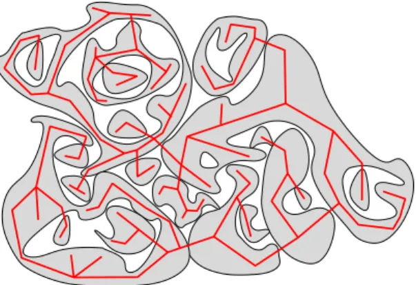
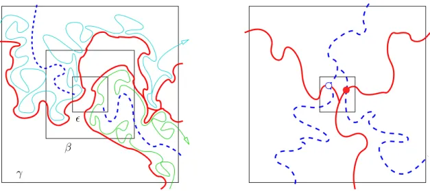
The MST in a box, and InvPerc started from the midpoint of the left boundary of the box until reaching the right boundary, onZ².

arXiv:1309.0269v3 [math.PR] 25 Jan 2017

(2)

1 Introduction

The Minimal Spanning Tree of weighted graphs is a classical combinatorial object [Bor26, Kru56, GrH85], and is also very interesting from the viewpoint of probability theory and statistical physics: when the weights on the edges of a graph are chosen at random, using i.i.d. variables, then the resulting random tree turns out to be closely related to the near- critical regime of Bernoulli bond percolation on that graph.

In Bernoulli bond percolation at density p ∈[0,1], each edge of the graph is kept open with probability p or becomes closed with probability 1−p, independently, and then one looks at the connected open components, called clusters. In site percolation, the vertices

(3)

are chosen to be open or closed instead of the edges. These are among the most important spatial stochastic processes, due to their simultaneous simplicity and richness [BrH57, Kes82, Gri99]. The main interest is in the phase transition near the critical densityp_c, below which all clusters are small, above which a cluster (sometimes clusters) of positive density emerge.

The theory of critical percolation in the plane has seen a lot of progress lately, starting with Smirnov’s proof of conformal invariance of crossing probabilities for site percolation on the triangular lattice [Smi01], and with the introduction of the Stochastic Loewner Evolution [Sch00] that describes the conformally invariant curves that are the scaling limits of interfaces between open and closed clusters. These SLE curves can be used to understand critical percolation in depth [Wer09], including the computation of critical exponents that had been predicted by physicists using non-rigorous conformal field theory techniques.

Beyond the static critical system, it is natural to consider dynamical versions: first, to slowly change p near pc and observe how the phase transition exactly takes place — called near-critical percolation; second, to apply a stationary dynamics and observe how the critical system is changing in time — called dynamical percolation. Indeed, by “perturbing”

critical percolation, the static results of the previous paragraph have also given way to an exhaustive study of dynamical and near-critical percolation [SchSt10, GPS10, HmPS15, GPS13a, GPS13b]; see also the surveys [Ste09, GaS12]. In particular, in [GPS13a, GPS13b]

we have proved the existence and conformal covariance of the scaling limit of the near- critical percolation ensemble, w.r.t. the quad-crossing topology introduced in [SchSm11].

Very roughly, this near-critical scaling limit is constructed from the critical scaling limit, plus independent randomness that governs how macroscopic clusters merge as we raisep.

It turns out that the macroscopic structure of the Minimal Spanning Tree (MST) and the Invasion Percolation Tree (InvPerc) can also be described based on this merging process.

Thus, building on [GPS13a, GPS13b], in the present paper we prove the existence and some conformal properties of the scaling limits of MST and InvPerc on the triangular lattice, in the space of essential spanning forests introduced in [AiBNW99]. In that paper, tightness results were proved, implying that subsequential scaling limits of the Minimal and Uniform Spanning Trees in the plane exist. Our proof of the uniqueness of the scaling limit has the important implication that the conjectural universality of critical percolation implies universality for many processes related to the near-critical ensemble, including MST and InvPerc. That this program of describing near-critical objects from the critical scaling limit may have a chance to work was suggested in [CFN06]. Another motivation for our work is that it leads to interesting new objects: these two scaling limits are invariant under rotations and scalings, but, conjecturally, not under general conformal maps. Furthermore, the methods developed to establish these scaling limits also give information about the large-scale geometry of the discrete trees.

1.1 The Minimal Spanning Tree MST

For each edge of a finite graph,e∈E(G), let U(e) be an independent Unif[0,1] label. The Minimal Spanning Tree, denoted by MST, is the spanning tree T for which P

e∈T U(e) is minimal. This is well-known to be the same as the union of lowest level paths between

(4)

all pairs of vertices (i.e., the path between the two points for which the maximum label on the path is minimal). One can also use the so-called reversed Kruskal algorithm to constructMST: delete from each cycle the edge with the highest labelU. This algorithm also shows that MST depends only on the ordering of the labels, not on the values themselves.

Moreover, this algorithm also makes sense on any infinite graph, and produces what in general is called the Free Minimal Spanning Forest (FMSF) of the infinite graph. The Wired Minimal Spanning Forest (WMSF) is the one when we also remove the edge with the highest label (if such edge exists) from each cycle that “goes through infinity”, i.e., which is the union of two disjoint infinite simple paths starting from a vertex. For the case of Euclidean planar lattices, these two measures on spanning forests are known to be the same, again denoted by MST, and it almost surely consists of a single tree [AleM94]. This measure can also be obtained as athermodynamical limit: take any exhaustion by finite subgraphs Gn(Vn, En), introduce a boundary condition by identifying some of the vertices on the boundary of G_n (i.e., elements of V_n that have neighbors in G outside of V_n), and then take the weak limit. On a general infinite graph, when no identifications are made in the boundary, one gets the FMSF, and when all vertices are glued into a single vertex, one gets theWMSF. Studying these measures has a rich history onZ^d, on point processes inR^d, and on general transitive graphs; see [Ale95, Pen96, Yuk98, AldS04, LPS06, Tim06, ChS13, Tim15, NTW15, LyP16] and the references therein.

One can use the same Unif[0,1] labels that defined the MST to obtain a coupling of percolation for all densitiesp∈[0,1]: an edge is “open at levelp” if U(e)≤p. This way we get acouplingbetween theMSTand thepercolation ensemble. Moreover, as we explain in the next paragraph, the macroscopic structure of theMSTis basically determined by the labels in the near-critical regime of percolation, and hence one may hope that the scaling limit of the MST is determined by the scaling limit of the near-critical ensemble.

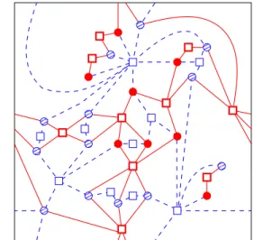
Figure 1.1: The MST connects the percolation p-clusters without creating cycles, yielding the cluster-tree MST^p.

Consider the p-clusters (i.e., open components at level p) in the percolation ensemble on some large finite graph. Contract each component into a single vertex, keeping the edges (together with their labels) between the clusters, resulting in the “cluster graph”. It is easy

(5)

to verify that making these contractions on theMSTwe get exactly the MSTon the cluster graph. We denote this cluster tree by MST^p. See Figure 1.1. Now assume that p₁ is small enough so that even the largestp₁-clusters are of small macroscopic size — then the tree MST^p¹ will tell us the macroscopic structure of MST. On the other hand, if p₂ > p₁ is large enough, then most sites are in just one giant p₂-cluster. Note that, for any p > p₁, we get the tree MST^p from MST^p¹ by contracting the edges with labels in (p₁, p]. Thus, if we have the collection of all the p-clusters for all p ∈ (p₁, p₂), then by following how they merge as we are raising p, we can reconstruct the tree MST^p¹. Now, one may hope that in order to tell the macroscopic structure ofMST^p¹, it is enough to know only themacroscopic p-clusters for all p ∈ (p1, p2) and follow how those merge. The near-critical window of percolation is exactly the window (p₁, p₂) in which the above phase transition of the cluster sizes takes place, and the scaling limit of the near-critical ensemble is exactly the object that describes the macroscopicp-clusters in this window. Therefore, the above hope has the interpretation that the scaling limit of the near-critical ensemble should describe the scaling limit of the MST. This, of course, raises several questions: May the dust of microscopic p-clusters condensate into a new macroscopic p⁰-cluster at somep⁰ > p, ruining the strategy of “following how macroscopic clusters merge”? Could MST^p¹ go through microscopic p₁- clusters in a way that significantly influences its macroscopic structure?

Our work addresses these questions in the case of planar lattices. The near-critical window for Bernoulli(p) percolation on the triangular lattice ηT or the square lattice ηZ² with mesh η >0 is given by

p= 1/2 +λr(η) with λ∈(−∞,∞) fixed and η→0, (1.1) where r(η) = η²/α₄(η,1), with α₄(η,1) being the alternating 4-arm probability of critical percolation [Wer09]. It was proved on ηT using SLE₆ computations [SmW01] that r(η) = η^3/4+o(1). As shown in [Kes87], forλ −1 we are at the subcritical end of the near-critical window, for λ 1 we are at the supercritical end, and for any fixed λ ∈ R, box-crossing probabilities are comparable to the critical case (just they are close to 0 for λ −1, and close to 1 for λ 1). That is, (1.1) is indeed the near-critical window. Then it was proved in [GPS13a, GPS13b] that for any λ ∈ R there is a unique scaling limit as η → 0;

moreover, the entire coupled percolation ensemble, viewed near the critical point via the parametrization (1.1), where all the macroscopic changes happen, has a scaling limit as a Markov process in λ ∈ R. It is important to keep in mind that even for any given λ 6= 0, this scaling limit is an interesting new object, known to be different from the critical scaling limit: the interfaces are singular w.r.t. SLE₆ [NoW09]. (See also [Aum14] and [GPS13b, Theorem 13.4] for the much simpler result that the full scaling limits are singular.)

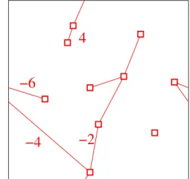
Since we have a proof of the existence and properties of the scaling limit of the near- critical ensemble only for site percolation on the triangular latticeT, if we want to use that to build theMSTscaling limit, we will need a version of theMST that uses Unif[0,1] vertex labels{V(x)}on T. So, assign to each edge e= (x, y) the vector label

U(e) := V(x)∨V(y), V(x)∧V(y)

, (1.2)

(6)

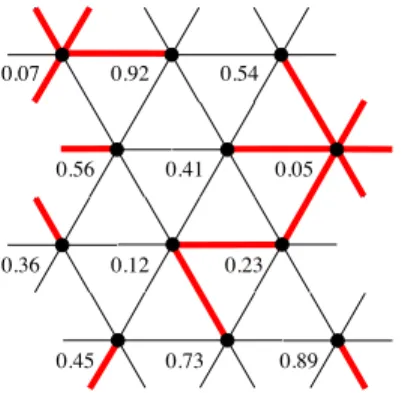
and consider the lexicographic ordering on these vectors to determine the MST. See Fig- ure 1.2. With a slight abuse of terminology, this is what we will call theMSTon the lattice T. Our strongest results will apply to this model, but some of them will also hold for subsequential limits of the usualMST onZ², known to exist by [AiBNW99].

0.56

0.07 0.92 0.54

0.05 0.41

0.23 0.36

0.89 0.73

0.12

0.45

Figure 1.2: The minimal spanning tree associated to vertex labels of the triangular lattice T, with a periodic boundary condition.

Let us make an important remark here. The use of the lexicographic ordering for the vector labels (1.2) is somewhat arbitrary, and starting from the same vertex labels, using a different way to get edge labels or using a different natural ordering, one could a priori get anMST with a very different global structure. In fact, this does happen if the vertex labels are assigned maliciously. Nevertheless, with the Unif[0,1] labels, for any rule to construct the MST on T that ensures that any two p-clusters are connected by a unique path of this MST (which is exactly how our definition works), our approximation of the macroscopic structure of theMST using the near-critical ensemble will work with large probability, and hence the scaling limit will be the same.

We can now state our main theorem:

Theorem 1.1 (Limit of MSTη in C). As η →0, the spanning tree MSTη on ηT converges in distribution, in the metric d_Ω of Definition 2.2 below, to a unique scaling limit MST∞

that is invariant under translations, scalings, and rotations.

The strategy of the proof will be described in Subsection 1.4. As a key step, we also prove convergence in any fixed torus T²M; see Theorem 5.1. We work in tori to avoid the technicalities related to boundary issues, but with not too much additional work the extension to finite domains with free or wired boundary conditions would be certainly doable.

In Section 6, strengthening the results of [AiBNW99], we study the geometry of the limiting treeMST_∞. The degree of a vertex in a tree graph has the usual meaning, but the degree of a point in a spanning forest of the plane needs to be defined carefully, which we will do in Subsection 6.1. To give an example, a pinching point on anMST∞path should not be called a branching point, but it still gives rise to a degree 4 point. Consequently, stating the results on the geometry of the limiting tree also needs some care, to be done precisely only in Theorem 6.2. Nevertheless, here are some of the earlier results and our new ones

(7)

in rough terms. It was proved in [AiBNW99] that there is an unspecified absolute bound k₀ such that almost surely all degrees in any subsequential limit of MST_η are at most k₀. Furthermore, the set of branching points was shown to be almost surely countable. Here, we will prove that there are almost surely no pinching points, all degrees are bounded by 4, and the set of points with degree 4 is at most countable. We will also prove, in Subsection 6.2, that the Hausdorff dimension of the trunk is strictly below 7/4. However, we do not have a guess for the exact dimension; the situation is similar to the somewhat related problem of finding the percolation chemical distance exponent [Dam16].

To conclude this subsection, let us note that the recent works [AdBG12, AdBGM13]

follow a strategy similar to ours, but in a very different setting: namely, in themean-field case. It is well-known that there is a phase transition at p = 1/n for the Erd˝os-R´enyi random graphsG(n, p). Similarly to the above case of planar percolation, it is a natural problem to study the geometry of these random graphs near the transitionpc= 1/n. It turns out in this case that the non-trivial rescaling is to work with p = 1/n+λ/n^4/3, λ ∈R. If R_n(λ) = (C_n¹(λ), C_n²(λ), . . .) denotes the sequence of clusters atp= 1/n+λ/n^4/3, ordered in decreasing order of size, say, then it is proved in [AdBG12] that asn → ∞, the normalized sequence n^−1/3R_n(λ) converges in law to a limiting object R∞(λ) for a certain topology on sequences of compact spaces which relies on the Gromov-Hausdorff distance. This near- critical ensemble{R_∞(λ)}_λ∈_R has then been used in [AdBGM13] to obtain a scaling limit as n→ ∞(in the Gromov-Hausdorff sense) of theMSTon the complete graph withn vertices.

One could say that [GPS13b] is the Euclidean (d = 2) analogue of the mean-field case [AdBG12], and our present paper is the analogue of [AdBGM13]. However, an important difference is that in the mean-field case one is interested in the intrinsic metric properties (and hence works with the Gromov-Hausdorff distance between metric spaces), while in the Euclidean case one is first of all interested in how the graph is embedded in the plane.

1.2 The Invasion Percolation Tree InvPerc

The connection betweenWMSF and critical percolation on infinite graphs can also be seen through invasion percolation. For a vertex x in an infinite graph G(V, E), and the labels {U(e)}, let T₀ = {x}, then, inductively, given T_n, let T_n+1 = T_n ∪ {e_n+1}, where e_n+1 is the edge between T_n and V \ T_n that has the smallest label U. The Invasion Percolation Tree of x is then InvPerc(x) := S

n≥0T_n. It is easy to see that, even de- terministically, if U : E(G) −→ R is an injective labelling of a locally finite graph, then WMSF=S

x∈V(G)InvPerc(x).

Once the invasion tree enters an infinite p-cluster C, it will not use edges outside it.

Furthermore, it is not surprising (though non-trivial to prove, see [H¨aPS99]) that for any transitive graph G and any p > p_c(G), the invasion tree eventually enters an infinite p- cluster. Therefore, lim sup{U(e) : e ∈ InvPerc(x)} = p_c(G) for any x ∈ V(G). This way, invasion percolation can be considered as a “self-organized criticality” version of critical percolation; finer results for the planar case are given in [CCN85, DSV09, DaS12]. Moreover, InvPerc can be used to study Bernoulli percolation itself: e.g., for the well-behavedness of

(8)

the supercritical phase on Z^d, d > 2 [CCN87], and for uniqueness monotonicity on non- amenable graphs [H¨aPS99]. Invasion percolation can be analyzed very well on regular trees [AnGHS08], with a scaling limit that can be described using diffusion processes [AnGM13].

For planar lattices, since InvPerc_η is so intimately related to MST_η, it will be quite easy to modify the proof of Theorem 1.1 for the case of InvPerc; see Section 7.

1.3 The scaling limit of the near-critical ensemble

We need to recall how the scaling limit of the near-critical ensemble is constructed in [GPS13a, GPS13b], because the present paper is heavily built on this. To start with, we slightly change the near-critical parametrization given in (1.1):

Definition 1.2. Thenear-critical ensemble (ω_η^λ)λ∈R will denote the following process:

(i) Sampleω_η^λ=0 according to P_η, the law of critical percolation onηT. We will sometimes represent this as a black-and-white coloring of the faces of the dual hexagonal lattice, with white hexagons standing for closed (empty) sites.

(ii) As λ increases, closed sites (white hexagons) switch to open (black) at an exponential rate r(η), as given after (1.1).

(iii) As λ decreases, black hexagons switch to white at rate r(η).

Note that, for anyλ∈R, the near-critical percolationω_η^λ corresponds exactly to a percolation configuration on ηT with parameter

(p=p_c+ (1−p_c) (1−e^{−λ r(η)}) if λ≥0 p=pce^−|λ|^r(η) if λ <0.

For any site x, the value λ(x) ∈ R where x switches from closed to open will be called the near-critical percolation label of x.

The same definitions can be made on ηZ².

It is easy to understand intuitively why r(η) is the right time rescaling to obtain the near-critical window. Assume that in the unit square there is no left-right crossing inω^λ=0_η . Then the expected number of those sites that are closed at λ = 0 but are pivotal for the left-right crossing (i.e., opening any of them would establish the crossing) and which actually become open in ω^λ_η is known to be of order λ. Therefore, for λ > 0 small, it is unlikely that a left-right crossing has been established if it was not already there, hence the system must have stayed very close to critical; on the other hand, one may expect that forλ 1 a crossing is already quite likely, hence the system should already be quite supercritical. This was rigorously proved in [Kes87]. Then, if one wants to describe the scaling limit of ω^λ_η as η → 0, a natural idea that was detailed in [CFN06] is that this should be possible by following which of those points get opened (for λ >0) or get closed (for λ <0) that were pivotal atλ= 0 for at least some small macroscopic distance >0. To this end, one should

(9)

look at the counting measure on -pivotal points at criticality, normalized such that the measure stays non-trivial asη →0, and hope that these-pivotal measures have limits that are measurable w.r.t. the scaling limit of critical percolation itself. This is the main result of [GPS13a] (with a slight change of what -pivotal means). Then, the scaling limit of the near-critical ensemble may be described by taking Poisson point processes of switch times, with intensity measures being these-pivotal measures, and by updating the crossings of all the quads (certain generalized rectangles) according to these pivotal switches. This is done in [GPS13b]. Here there are roughly two main issues: firstly, it is not immediately clear how one can update the crossings of all the quads by pivotal switches that are happening atall spatial and time scales. For this, one should code the percolation configuration in a suitable manner that is minimal enough so that the updates can be done, but rich enough so that it contains all the relevant information. This coding and updating takes up a large part of [GPS13b], done through the so-called -networks that we will actually recall in Section 3. The second main issue is that one needs to prove that despite all the switches that take place asλincreases, following the switches of all the initially-pivotal sites gives a good idea about the -pivotal switches at later times. For this, the key discrete result from [DSV09, GPS13b] is the following proposition, which we will often use also in the present paper:

Proposition 1.3 (Near-critical stability). For any fixed −∞ < λ < λ⁰ < ∞, in the near- critical ensemble onηT, letA^λ,λ_k ⁰(r, R) denote the following near-critical polychromatic k-arm event: there exist k ≥2 disjoint paths in the lattice that connect the boundary pieces of the annulusB_R(0)\B_r(0), each called either “primal” or “dual”, and all the percolation ensemble labels along all the primal arms are at most λ⁰, while all the labels along the dual arms are at least λ. Note that λ =λ⁰ gives back the usual notion of primal and dual arms in the percolation configuration ω^λ_η. Then,

P

A^λ,λ_k ⁰(r, R)

≤C_λ,λ⁰α_k(r, R),

where αk(r, R) = α^η_k(r, R) is the polychromatic k-arm probability in critical percolation on the same lattice. Similarly, for themonochromatick-arm events, k≥1, where all arms are primal,

P

A^λ_k⁰(r, R)

≤C_λ,λ⁰ 0α⁰_k(r, R),

whereα⁰_k(r, R) = α^0η_k(r, R)is the monochromatick-arm probability at criticality. Forα₁⁰(·,·), we will just use α₁(·,·).

The same statements hold for bond percolation on ηZ², just with dual arms being paths in the dual lattice, in the usual manner.

Remark 1.4. For fixed radii 0 < r < R < ∞, the discrete multi-arm probabilities α^η_k(r, R) and α^0η_k(r, R) converge, asη →0, to their SLE₆ counterparts (see [Wer09]). In the present paper, we will be interested in these quantities only up to constant factors, not in the details of their convergence, hence their dependence onηis not important and will be omitted from the notation. Formulas like α_k(η,1) will also be understood on the discrete lattice, always

(10)

with mesh η. We will also use the quasi-multiplicativity of multi-arm probabilities (both for the discrete and continuum versions): for anyk ≥1, there exists c_k >0 such that

c_kα_k(r₁, r₂)α_k(r₂, r₃)≤α_k(r₁, r₃)≤α_k(r₁, r₂)α_k(r₂, r₃),

for all 0< r1 < r2 < r3 <∞. Similarly for α⁰_k. See, e.g., [Nol08, Subsection 4.5].

The proof of Proposition 1.3 for the alternating 4-arm event is given in [DSV09, Lemma 6.3], or follows directly from [GPS13b, Lemma 8.4], which is more general in that it does not assume that the dynamics is monotone inλ. For general k, the case ofλ =λ⁰ is known as Kesten’s near-critical stability [Kes87]. And just as in Kesten’s approach, the proof for general k and general λ < λ⁰ is a simple modification of the proof for the alternating 4- arm event: the key point is that the pivotality of a site for a generalk-event still depends on an alternating 4-arm event around that site, and hence the near-critical stability of the alternating 4-arm probability, proved using a recursion in [GPS13b], easily implies the stability of the general k-arm event, as well. We omit the details.

The above sketch of the contents of [GPS13a, GPS13b] should make it clear that the scaling limit of the near-critical ensemble is constructed entirely from the critical scaling limit, plus independent randomness of the pivotal switch times. Moreover, all the proofs in [GPS13a, GPS13b] are universal in the sense that they use lattice-independent discrete percolation technology that have been available since [Kes87]. Altogether, once one proves Cardy’s formula for critical percolation on ηZ², which would imply the same scaling limit as on ηT, we would also immediately get that the scaling limit for the entire near-critical ensemble is the same. This universal aspect remains true for the present paper.

1.4 Strategy of the proof and organization of the paper

First of all, in Subsection 2.1, we describe the topological space in which the convergence of our random trees will take place: the space of essential spanning forests inC, introduced in [AiBNW99]. There are possible alternatives to using this topology, such as the quad-crossing topology of [SchSm11] (suggested to us for this purpose by Nicolas Broutin) or the topology introduced in [Sch00] for the scaling limit of the Uniform Spanning Tree. Especially the quad-crossing topology (recalled in Subsection 2.2) would seem natural, since the scaling limit of near-critical percolation is taken in this space. Nevertheless, we chose the topology of [AiBNW99] for several reasons: that was the first paper dealing with subsequential scaling limits ofMST_η, proving results that we are sharpening here; using this topology to describe paths in the spanning trees is not harder than using quad-crossings, while it also gives a natural way to glue the paths into more complicated trees; there is a simple explicit metric generating this topology. However, we will unfortunately need more topological preparations than just recalling these definitions, because the minimalist structure, based on just the pivotal measures of [GPS13a], which was enough to describe the scaling limit of the near-critical ensemble in [GPS13b], will not be enough for the tree structures of the present paper. In particular, in Proposition 2.6, we will prove that that set of colored pivotals also has a limit asη →0.

(11)

In Section 3, we first recall the definition of the networks N^¯^λ,_η and N^λ,_∞^¯ introduced in [GPS13b], where ¯λ = (λ, λ⁰) is a pair of near-critical parameters with λ < λ⁰. These are graphs with vertex sets X given by those-pivotals in the configuration ω^λ on a torusT²M

that experience a switch between levelλand λ⁰, and edges given roughly by the primal and dual connections in ω^λ\X. Then we need to add a bit more structure to these networks, creating the so-calledenhanced networks: roughly, we will need to know which of these pivotals are connected together by an open cluster of ω^λ \X, and will need to know the colors of these pivotals inω^λ. For this, we will use Proposition 2.6 mentioned in the previous paragraph and Proposition 3.6 saying that clusters of large diameter also have large volume (which excludes certain pathological geometric behaviour that would ruin the construction).

From these enhanced networks, we will obtain finite labelled graphs whose vertices will basically be open λ-clusters that have -pivotals switching in the time interval (λ, λ⁰), with edges labelled by the times of the pivotal switches, showing how the λ-clusters merge. We will define the MST on this finite labelled graph, denoted by MST^λ,_η^¯ in the discrete and MST^¯^λ,_∞ in the continuum case — these are basically the macroscopic approximations to the cluster trees that we discussed in Subsection 1.1. To be more precise, in Section 3 we define only some Minimal Spanning Forests, and we need a bit more work until in Lemma 4.4 we can actually define the trees. The fact that these approximatingcut-off trees MST^¯^λ,_η and MST^¯^λ,_∞ are close to each other if the underlying near-critical ensemblesωη^[λ,λ⁰^]and ω^[λ,λ∞ ⁰^] are close follows easily from [GPS13b].

In Section 4 we prove that the cut-off treesMST^¯^λ,_η are close to the trueMST_η ifλ −1, λ⁰ 1, and >0 is small. Here the key technique is near-critical stability, Proposition 1.3.

Summarizing, we get that MST_η is close toMST^λ,_∞^¯ . Since the latter does not depend on η, while the former does not depend on ¯λ and , they both need to be close to an object that does not depend on any of these parameters: this will be the scaling limit MST_∞. To give a succinct pictorial summary of this strategy:

MST_η MST^¯^λ,_η MST^λ,_∞^¯

MST_∞

This conclusion will be materialized in Section 5, together with the extension from the case of the toriT²M to the full plane, and with the proof of the claimed invariance properties.

As already advertised in Subsections 1.1 and 1.2, the results on the geometry of MST∞

are discussed in Section 6, while Section 7 establishes the existence and invariance properties of InvPerc_∞. We conclude the paper with some open problems in Section 8.

Acknowledgments. We thank Louigi Addario-Berry, Nicolas Broutin, Laure Dumaz, Gr´egory Miermont and David Wilson for stimulating discussions, Rob van den Berg for pointing out the connection between Proposition 3.6 and [J´ar03], and Alan Hammond and two amazing anonymous referees for very good comments on the manuscript.

(12)

Part of this work was done while all authors were at Microsoft Research, Redmond, WA, or GP was visiting CG at ENS Lyon. CG was partially supported by the ANR grant MAC2 10-BLAN-0123. GP was supported by an NSERC Discovery Grant at the University of Toronto, an EU Marie Curie International Incoming Fellowship at the Technical University of Budapest, and partially supported by the Hungarian National Research, Development and Innovation Office, NKFIH grant K109684, and by the MTA R´enyi Institute “Lend¨ulet”

Limits of Structures Research Group.

2 Topological and measurability preliminaries

2.1 The space of essential spanning forests

The following topological setup for discrete and continuum spanning trees was introduced in [AiBNW99]. We are summarizing here the definitions and the notation, with small modifications; the main difference is roughly that Ω will also contain spanning trees of subsets of the complex plane, to accommodate the invasion percolation treeInvPercand our approximating trees MST^¯^λ,.

We will work in a one-point compactification of C=R², denoted by ˆC=C∪ {∞}, with the Riemannian metric

4

(1 +x²+y²)² dx² +dy²

; (2.1)

by stereographic projection, ˆC is isometric with the unit sphere. Note that this metric is equivalent to the Euclidean metric in bounded domains, while the distance between any two points outside the square of radiusM around the origin in Cis at most O(1/M). This will imply that convergence of spanning trees in ˆC is the same as convergence within bounded subsets of C. This is necessary, since convergence of random spanning trees cannot be uniform inC: on ηZ², inside the infinitely many pieces [i, i+ 1)×[j, j+ 1),i, j ∈Z, one can find arbitrary topological behavior (e.g., macroscopically vanishing areas with arbitrarily large numbers of macroscopic branches emanating from them) that will be very far from the almost sure behavior of the continuum tree.

Spanning trees on infinite graphs are usually defined and studied as weak limits of spanning trees in finite subgraphs exhausting the infinite graph. For these finite graphs, one may consider different boundary conditions: most importantly, free or wired. As mentioned in the Introduction, for theMST on Euclidean planar lattices, all such boundary conditions give the same limit measure, and we will work in the toriT²M of side-length 2M, which can be realized as the subdomains [−M, M)² ofC, or even as subgraphs ofηTfor suitable values of M, with a periodic boundary condition (which is sandwiched between the free and the wired conditions). See Figure 1.2 in the Introduction.

Definition 2.1. Areference treeτ is a tree with a finite set of leaves (or external vertices), denoted by ξ(τ), with each edge considered to be a unit interval. A reparametrization is a continuous map φ : τ −→ τ that fixes all the vertices and is monotone on the edges.

(13)

An immersed tree indexed by τ is an equivalence class of continuous maps f : τ −→

Cˆ, where f₁ and f₂ are considered equivalent if there exist reparametrizations φ₁, φ₂ with f₁◦φ₁ =f₂◦φ₂. The collection of immersed trees indexed by τ is denoted by S_τ, and we set

S^(`):= [

τ:|ξ(τ)|=`

S_τ. (2.2)

Immersed trees with leavesx₁, . . . , x_` ∈Cˆ will often be denoted by T(x₁, . . . , x_`)∈ S^(`). We will also consider trees immersed into the torus T²M with the flat Euclidean metric;

the corresponding collection of immersed trees with ` leaves is denoted by S_M^(`).

One may consider trees immersed not just into Cˆ or T²M, but into a graph G(V, E) that is embedded into Cˆ or T²M, and then the image of τ is required to be a subtree of G(V, E), with its vertices mapped into V and any of its edges mapped to a union of edges from E.

τ ξ₁

ξ₂ ξ₃

ξ₄

x1

x₂ x₃

x₄

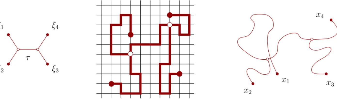
Figure 2.1: A reference tree τ with four leaves, with one immersion into Z² and another intoC. TheimageinCis not a tree, but this is allowed. In the scaling limit of any discrete random tree in ˆC one cannot see such self-intersections, but could see touch-points, and self-intersections might happen in scaling limits in higher dimensions.

Note that if a reference tree τ⁰ is given by contracting some edges of some τ, denoted by τ⁰ ≺ τ, then Sτ⁰ is naturally a subset of Sτ, represented by maps f : τ −→ Cˆ that are constants on the contracted edges. By contractions in two non-isomorphic trees,τ₁ and τ₂, we may reach the same tree τ⁰ ≺ τ_i, hence S^(`) may be viewed as covered by patches S_τ that are sewn together along “smaller dimensional” patches Sτ⁰, similarly to a simplicial complex. (In particular, after these identifications, (2.2) stops being a disjoint union.)

We now equip each S_τ with a very natural metric, extending the notion of uniform closeness up to reparametrization of curves: for two immersed treesf1, f2 :τ −→Cˆ,

dist_τ(f₁, f₂) = inf

φ1,φ2

sup

t∈τ

dist_ˆ

C f₁◦φ₁(t), f₂◦φ₂(t)

, (2.3)

where theφ_i’s run over all reparametrizations ofτ. This can be easily extended to immersed trees indexed by different reference trees: by the above remark about patches, for any pair

(14)

of reference trees τ, τ⁰ there exist sequences τ = τ₀, τ₁, . . . , τ_m = τ⁰ such that τ_i ≺ τ_i+1 or τ_i τ_i+1 for alli= 0, . . . , m−1, and then for anyf :τ −→Cˆ andf⁰ :τ⁰ −→Cˆ we can take dist(f, f⁰) = inf

(_m−1 X

i=0

dist_τ_i_gτ_i+1(f_i, f_i+1) :f₀ =f, f_m =f⁰, τ_i−→^fⁱ Cˆ for i= 1, . . . , m−1 )

,

where, with a rather obvious notation, τi gτj = τi if τi τj. For instance, for any τ, τ⁰ there exists τ⁰⁰ with τ, τ⁰ ≺τ⁰⁰, hence dist(f, f⁰)≤dist_τ⁰⁰(f, f⁰).

With this metric, S^(`) is clearly a complete separable metric space, called the space of

`-trees. Of course, a Cauchy sequence of trees contained fully inC might have a limit that has an edge going through∞. Similarly, S_M^(`) is complete and separable with the analogous metric, just using the Euclidean metric onT²M in (2.3).

Now that we have a definition for the space of finite trees immersed in ˆC orT²M, we can start defining what a spanning tree of ˆC or T²M should be: a set of finite trees that satisfy certain compatibility conditions.

The set of non-empty closed subsets of S^(`) in the above metric, equipped with the Hausdorff metric, is denoted by Ω^(`). We will consider graded sets

F = F^(`)

`≥1 ∈ Ω^× := X

`≥1Ω^(`),

with the product topology. Clearly, Ω^× is again complete, separable and metrizable; in one word, it is a Polish metric space.

Extending the map τ 7→ ξ(τ) giving the external vertices of an index tree, for any F ∈Ω^× we can define

ξ(F) := [ n

f(ξ(τ)) :τ−→^f Cˆ ∈ F^(`), `≥1o

⊂Cˆ,

which gives the set of external vertices occurring in F. It is clearly a Borel measurable function, since for any open U ⊂Cˆ, the preimage ξ⁻¹(U) is a countable intersection (over

`≥1) of open sets.

Let SB1,...,B_` be the set of immersed trees with endpoints xi ∈ Bi, where each Bi is a closed subset of ˆC. Note that this is a closed subset of S^(`). The non-empty closed subsets of S^(`) that do not intersect S_B₁_,...,B_` form an open set in the Hausdorff metric, hence the map

Ω^× −→Ω_B₁_,...,B_` ⊆Ω^(`), F 7→ F^(`)∩ S_B₁_,...,B_`

is measurable. In words, extracting the subtrees ofF with leaves in prescribed closed sets (e.g., the branches ofF connecting two given points) is a measurable map.

Definition 2.2. A graded setF = F^(`)

`≥1 ∈Ω^× is called an essential spanning forest on its external vertices ξ(F) if it satisfies the following properties:

(i) for each ` ∈ N⁺ and any `-tuple {x₁, . . . , x_`} of vertices in ξ(F), there exists at least one immersed tree T(x₁, . . . , x_`)∈ F^(`) with those leaves;

(15)

(ii) for any immersed treeT ∈ F^(`), any subtreeT⁰ ⊂T (given by restricting the immersion to a combinatorial subtree of the index tree τ) is again in some F^(`⁰⁾;

(iii) for any two trees T_i ∈ F^(`ⁱ⁾, i = 1,2, there is a tree in some F^(`) that contains both T_i’s as subtrees and has no leaves beyond those of the T_i’s.

Note that (ii) implies that ξ(F) contains all the vertices of all the embedded trees.

An essential spanning forest F is called a spanning tree if ξ(F) ⊂ C and every path T(x, y)∈ F⁽²⁾ stays within a bounded region of C. A spanning tree is called quasi-local if for any bounded Λ ⊂C there exists a bounded domain Λ(F¯ ,Λ)⊂C such that every tree of F with leaves in Λ is contained in Λ.¯

The set of essential spanning forests in Cˆ (with an arbitrary set of vertices ξ(F)) will be denoted by Ω. It is easy to check that Ω is a closed subset of the Polish space Ω^×, hence itself is Polish. A simple explicit metric, denoted by d_Ω, is given by the restriction from Ω^× to Ω of the sum over ` of the Hausdorff distance on S^(`) multiplied by the weight 2^−`.

For the toriT²M, the spacesΩ^(`)_M,Ω^×_M,Ω_M are defined analogously, with the only difference being that any essential spanning forest here is a single tree. The metric d_Ω_M is defined the same way as d_Ω.

The only way in which two vertices may be disconnected in an essential spanning forest F in ˆC is that all the paths between them go through ∞; therefore, either F is a spanning tree, or no component of it is contained in a bounded domain of C. This is the property that the adjective “essential” for these spanning forests refers to. (In the setting of discrete infinite graphs, this reduces to saying that all components of the forest are infinite trees.) Also, note that the above definition allows for having more than one path between two vertices, which will in fact happen in the scaling limit of theMST.

2.2 The quad-crossing topology

Let us quickly recall the notation and the basic results for the quad-crossing topology of percolation configurations, introduced in [SchSm11] and studied further in [GPS13a, GPS13b].

Let D ⊂ Cˆ = C∪ {∞} be open, or be equal to the torus T²M. A quad in the domain D can be considered as a homeomorphism Q from [0,1]² into D. The space of all quads in D, denoted by Q_D, can be equipped with the following metric: dQ(Q₁, Q₂) :=

inf_φsup_z∈∂[0,1]2|Q₁(z) − Q₂(φ(z))|, where the infimum is over all homeomorphisms φ : [0,1]² −→ [0,1]² which preserve the 4 corners of the square. A crossing of a quad Q is a connected closed subset of [Q] := Q([0,1]²) that intersects both ∂₁Q= Q({0} ×[0,1]) and ∂₃Q =Q({1} ×[0,1]). We say that Q has a dual crossing between ∂₁Q and ∂₃Q by some closed subset S ⊆[Q] if there is no crossing in S between ∂2Q =Q([0,1]× {0}) and

∂₄Q=Q([0,1]× {1}).

From the point of view of crossings, there is a natural partial order on Q_D: we write Q₁ ≤ Q₂ if any crossing of Q₂ contains a crossing of Q₁. Furthermore, we write Q₁ < Q₂ if there are open neighborhoods N_i of Q_i (in the uniform metric) such that N₁ ≤N₂ holds

(16)

for anyN_i ∈ N_i. A subset S ⊂ Q_D is called hereditary if whenever Q ∈S and Q⁰ ∈ Q_D satisfiesQ⁰ < Q, we also haveQ⁰ ∈S. The collection of all closed hereditary subsets of Q_D will be denoted byHD. Any discrete percolation configurationω_η of meshη >0, considered as a union of the topologically closed percolation-wise open hexagons in the plane, naturally defines an element S(ω_η) of HD: the set of all quads for which ω_η contains a crossing. In particular, near-critical percolation at level λ ∈ R, as defined in Definition 1.2, induces a probability measure onHD, which will be denoted by P^λ_η.

By introducing a natural topology,HD can be made into a compact metric space. Indeed, let

^Q :={S∈HD :Q∈S} for any Q∈ QD, and let

U :={S ∈HD :S∩U =∅} for any openU ⊂ Q_D.

Then, defineT_D to be the minimal topology that contains every^cQand ^c_U as open sets. It is proved in [SchSm11, Theorem 3.10] that for any nonempty openD, the topological space (HD,T_D) is compact, Hausdorff, and metrizable. Furthermore, for any dense Q₀ ⊂ Q_D, the events{Q :Q∈ Q₀}generate the Borelσ-field ofHD. An arbitrary metric generating the topology T_D will be denoted by d_H. Now, since Borel probability measures on a compact metric space are always tight, we have subsequential scaling limits of P^λ_η on HD, as η = η_k →0. Moreover, the following convergence of probabilities holds. For critical percolation, λ = 0, it is Corollary 5.2 of [SchSm11]; for general λ, the exact same proof works, using that the RSW estimates hold in near-critical percolation.

Lemma 2.3. For any λ ∈ R, any subsequential scaling limit P^λ_η

k → P^λ_∞, and any quad Q∈ Q_D, one has P^λ_∞[∂Q] = 0. Therefore, by the weak convergence of P^λ_η

k to P^λ_∞, P^λ_η

k[Q]→P^λ_∞[Q].

For the case of site percolation on ηT, we know much more than just the existence of subsequential limits. As explained in [GPS13a, Subsection 2.3], the existence of a unique quad-crossing scaling limit for λ = 0 follows from the loop scaling limit result of [Smi01, CaN06]. The case of generalλ is Theorem 1.4 of [GPS13b]:

Theorem 2.4 (Near-critical scaling limit). For any λ ∈ R, there is a unique measure P^λ_∞ for percolation configurations ω_∞^λ in (HD,T_D) such that the weak convergence ω^λ_η −→^d ω_∞^λ holds.

We have shown in [GPS13a] that the arm events between the boundary pieces of an annulus are measurable w.r.t. the quad-crossing topology, and the convergence of probabilities (analogous to Lemma 2.3) holds. Namely, for any topological annulus A ⊂ D with piecewise smooth inner and outer boundary pieces ∂₁A and ∂₂A (and for the case of D =T²M, we also requireA to be null-homotopic), we define the alternating 4-arm event inA as A₄ =S

δ>0A^δ₄, where A^δ₄ is the existence of quads Q_i ⊂D,i = 1,2,3,4, with the following properties (see the left side of Figure 2.2):

(17)

(i) Q₁ andQ₃ are disjoint and are at distance at leastδ from each other; the same forQ₂ and Q₄;

(ii) for i ∈ {1,3}, the sides ∂₁Q_i = Q_i({0} ×[0,1]) lie inside ∂₁A and the sides ∂₃Q_i = Qi({1} ×[0,1]) lie outside ∂2A; for i ∈ {2,4}, the sides ∂2Qi = Qi([0,1]× {0}) lie inside ∂₁A and the sides∂₄Q_i =Q_i([0,1]× {1}) lie outside ∂₂A; all these sides are at distance at least δ from the annulusA and from the other Q_j’s;

(iii) the four quads are ordered cyclically around A according to their indices;

(iv) For i ∈ {1,3}, we have ω ∈ ^Qi, while for i ∈ {2,4}, we have ω ∈ ^cQi. In plain words, the quads Q₁, Q₃ are crossed, while the quads Q₂, Q₄ are dual crossed between the boundary pieces of A, with a margin δ of safety.

The definitions of general(mono- or polychromatic)k-arm eventsinAare of course analogous: for arms of the same color we require the corresponding quads to be completely disjoint, and we still require all the boundary pieces lying outside the annulus A to be disjoint.

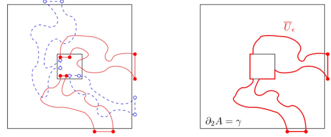
∂₂A=γ

U

Figure 2.2: Defining the alternating 4-arm event (in Subsection 2.2) and the color of a pivotal point (in Subsection 2.3) using quad-crossings. Quads with a primal crossing are in solid red, quads with a dual crossing are in dashed blue.

The following lemma is proved for critical percolation in Lemma 2.9 of [GPS13a]. For near-critical percolation, the same proofs work, using the stability of multi-arm probabilities (see Lemma 8.4 and Proposition 11.6 of [GPS13b], or [Kes87]), together with the existence of the near-critical scaling limit [GPS13b, Theorem 1.4].

Lemma 2.5. Let A⊂Dbe a piecewise smooth topological annulus (with finitely many non- smooth boundary points). Then the 1-arm, the alternating 4-arm and any polychromatic 6-arm event inA, denoted by A₁, A₄ andA₆, respectively, are measurable w.r.t. the scaling limit of critical percolation in D, and one has

η→0limP^λ_η[A_i] =P^λ_∞[A_i].

(18)

Moreover, in any coupling of the measures {P^λ_η} and P^λ_∞ on (HD,T_D) in which ω_η^λ →ω_∞^λ a.s. as η→0, we have

P

{ω_η^λ ∈ A_i}4{ω_∞^λ ∈ A_i}

→0 (as η→0). (2.4)

2.3 Pivotals and pivotal measures

In [GPS13b], we managed to describe the changes of macroscopic connectivities in a percolation configuration under the stationary or the asymmetric near-critical dynamics using just the pivotal measures of [GPS13a], without making explicit use of notions like clusters or the set of pivotal sites in continuum percolation. Unfortunately, the situation is slightly more complicated for the models in the present paper, hence we need some foundational work in addition to what was done in [GPS13a, Section 2.4].

Let x be a point surrounded (with a positive distance) by a piecewise smooth Jordan curve γ ⊂ D, where “surrounded” means that D\γ has two connected components, with the one containing x being homeomorphic to a disk. For any > 0, fix a lattice Z² in D, and let B(x) be the -square [i, i+ 1)×[j, j + 1) in the lattice that contains x. We say that x is pivotal for γ in ω^λ_∞ if, for any > 0 such that B(x) is surrounded by γ, the alternating 4-arm event occurs in the annulus with boundary pieces ∂B(x) and γ, as defined in Subsection 2.2. We let P^γ denote the set of pivotal points for γ in D.

Furthermore, we can identify thecolor of a pivotal point x∈ P^γ as open(black) versus closed (white, empty), as follows. We let P_open^γ, denote the set of points x for which γ surroundsxwithout intersecting or touchingB(x), and there exist quadsQ_,i,i= 1,2,3,4, exhibiting the 4-arm event from ∂B(x) to γ such that the quad U, given by taking the union ofU :=Q_,1∪Q_,3∪B(x) and the bounded components ofC\U, is crossed between the boundary piecesQ_,1({1} ×[0,1]) and Q_,3({1} ×[0,1]); see the right side of Figure 2.2 in the previous subsection. Then, we let the set of open pivotals forγ be

P_open^γ :=

x∈D:x∈ P_open^γ, for all >0 s.t. B(x) is surrounded by γ .

Clearly, the event x ∈ P_open^γ is measurable w.r.t. the quad-crossing topology. We will use the notation x∈ P_open^γ,,δ for the event that all the crossing events in P_open^γ, are satisfied even with aδ margin of safety. Finally, we set x∈ P_closed^γ if the analogous dual crossing holds in the quad given byQ_,2∪Q_,4∪B(x), for each small enough >0.

Note that for a discrete percolation configuration ω_η^λ the above definitions do not work:

instead of taking all small enough > 0, we just need to take the annulus between γ and the hexagon of the pointx∈D. And here it is clear what the setsP_open^γ (ω^λ_η) and P_closed^γ (ω^λ_η) are: their disjoint union is the set of pivotal hexagonsP^γ(ω_η^λ), and the color is determined by the color of the hexagon itself. We will also use notation like x∈ P_open^γ, (ω_η^λ): it has the meaning given above, using quad-crossings, and of course it cannot hold unless η is small enough, say >2η, so that ∂B(x) already intersects at least fourη-hexagons.

Proposition 2.6 (The set of pivotals, with colors). In any coupling of the measures {P^λ_η} and P^λ_∞ on (HD,T_D) in which ω^λ_η −−→^a.s. ω_∞^λ as η → 0, for any piecewise smooth null- homotopic Jordan curve γ ⊂D we have the following statements:

(19)

(i) P_open^γ (ω_η^λ)converges in probability to P_open^γ (ω_∞^λ )in the Hausdorff metric of closed sets.

Same for P_closed^γ .

(ii) Almost surely, P_open^γ (ω_∞^λ )∪ P_closed^γ (ω^λ_∞) = P^γ(ω_∞^λ ), a disjoint union.

(iii) Almost surely, whenever x ∈ P^γ(ω_∞^λ) for some γ, the color of x is the same for all such γ.

Note that (ii) is not a tautology (neither that the two colored sets are disjoint, nor that their union is the set of all the pivotals), since in ω^λ_∞ we did not define the set of closed pivotals as the complement of open pivotals.

The main difficulty in proving (i) is that the event x ∈ P_open^γ is not an open set in the quad-crossing topology (HD,T_D): perturbing a configuration even by an arbitrary small amount may destroy a pivotal for γ, making the 4-arm event happen only from a strictly positive distance > 0 to γ. In terms of discrete percolation configurations, if there is an open pivotal connecting two halves of a cluster, then making the connection between the two halves a bit thicker is a small change w.r.t. the quad-crossing topology, but it kills the pivotal. In particular, the harder direction in (i) will be to prove that there are “enough”

pivotals inω_∞^λ , since this requires controlling all scales simultaneously.

Proof. For (i), we need to prove that for any > 0, if η > 0 is small enough, then with probability at least 1−, for every x_η ∈ P_open^γ (ω_η^λ) there exists some x∈ P_open^γ (ω_∞^λ ) within distance fromx_η, and vice versa, for everyx∈ P_open^γ (ω^λ_∞) there exists x_η ∈ P_open^γ (ω_η^λ).

There will be two key ingredients. Firstly, for any small α, > 0 there exists δ,η >¯ 0 such that for all 0< η <η,¯

P

P_open^γ, (ω^λ_η) = P_open^γ,,δ(ω^λ_η)

>1−α . (2.5)

The existence of a δ that still depends on x ∈ P_open^γ, (ω^λ_η), or rather on its lattice square B(x), is just a special case of [GPS13a, Corollary 2.10]. Then, taking the probability α of the error much smaller than ², we can find a δ >0 that, with large probability, works for all points inP_open^γ, (ω^λ_η) simultaneously, proving (2.5).

The point of introducing theδmargin of safety is that now (2.5) immediately implies that there exists some monotone function f = f_α, : [0,∞) −→ [0,∞) that could be described using the dyadic uniformity structures of [GPS13a, Lemma 2.5] and [GPS13b, Proposition 3.9]) such that

P

∀x∈ P_open^γ, (ω^λ_η) and ∀ω˜ ∈HD with d_H(˜ω, ω^λ_η)< f(δ), we have x∈ P_open^γ,,δ/2(˜ω)