arXiv:1609.09746v1 [math.CO] 30 Sep 2016
INDEPENDENT SETS IN THE UNION OF TWO HAMILTONIAN CYCLES
RON AHARONI AND DANIEL SOLT´ESZ
Abstract. Motivated by a question on the maximal number of vertex disjoint Schrijver graphs in the Kneser graph, we investigate the following function, denoted by f(n, k):
the maximal number of Hamiltonian cycles on annelement set, such that no two cycles share a common independent set of size more thank. We shall mainly be interested in the behavior off(n, k) whenkis a linear function ofn, namelyk=cn. We show a threshold phenomenon: there exists a constant ct such that for c < ct, f(n, cn) is bounded by a constant depending only on c and not onn, and for ct < c, f(n, cn) is exponentially large inn (n→ ∞). We prove that 0.26< ct <0.36, but the exact value of ct is not determined. For the lower bound we prove a technical lemma, which for graphs that are the union of two Hamiltonian cycles establishes a relation between the independence number and the number ofK4subgraphs. A corollary of this lemma is that if a graphG onn >12 vertices is the union of two Hamiltonian cycles andα(G) =n/4, thenV(G) can be covered by vertex-disjointK4 subgraphs.
1. Introduction
In this paper we study a “pigeonhole” phenomenon for Hamiltonian cycles - in a large enough set of such cycles there are necessarily two that are close, in the sense that their union contains a large independent set (meaning that they are similar to each other).
The motivation comes from Schrijver subgraphs of the Kneser graph. The Kneser graph KG[n, k] has as vertices the k-subsets of [n], two vertices being connected if the sets are disjoint. A celebrated result of Lov´asz [7] is that the chromatic number of KG[n, k] is n−2k+ 1. His proof used topology, and it gave birth to the field of topological com- binatorics. Later Schrijver proved that a relatively small induced subgraph of KG[n, k]
already has the same chromatic number. The vertices of this subgraph are those k-sets that are independent on a given, fixed, Hamiltonian cycle on [n]. The question we are interested in is what is the largest size of a set of vertex disjoint Schrijver subgraphs of KG[n, k]. Two Schrijver subgraphs are vertex disjoint if their Hamiltonian cycles do not share an independent set of size k, meaning that the union of their Hamiltonian cycles has independence number less than k. So, the question is on the maximal number of Hamiltonian cycles with a given bound on the independence number of each pairwise union.
Throughout the paper, unless otherwise stated the size of the vertex set of any graph mentioned is denoted by n. As usual, α(G) denotes the maximal size of an independent set in a graph G. IfG and H are graphs on the same ground set V, we write G∪H for the graph on V with E(G)∪E(H) as edge set. A Hamiltonian cycle on V is a simple cycle containing all vertices of V.
Key words and phrases. Independent set, Hamiltonian cycle, union, threshold.
The research of the first author was supported by BSF grant no. 2006099, by GIF grant no. I−879− 124.6/2005, by the Technion’s research promotion fund, and by the Discont Bank chair.
The research of the second author was supported by the Hungarian Foundation for Scientific Research Grant (OTKA) No. 108947.
1
Definition 1.1. f(n, k) is the maximal size of a set H of Hamiltonian cycles on n vertices, such that α(H1∪H2)≤k for every H1 6=H2 ∈ H.
We study f(n, k) in the case where k is a linear function of n, namely k = cn. This is very natural as the independence number of a Hamiltonian cycle grows roughly like a linear function of n. Our main observation is the following threshold phenomenon.
Theorem 1.2. There is a constant ct, such that for c < ct the function f(n, cn) is bounded, and for ct< c the function f(n, cn) is exponentially large in n.
If H is a Hamiltonian cycle, then α(H) = ⌊n2⌋. Given two Hamiltonian cycles H1
and H2, their common independence number, α(H1 ∪H2), lies between n4 (this bound follows from Brooks’ theorem) and n2. Thus, the trivial bounds for the threshold are 0.25≤ct≤0.5. We improve these as follows.
Theorem 1.3.
0.26627≈ 45
169 ≤ct≤ 11
30 ≈0.3666.
Definition 1.4. A graph is said to betwo-miltonian if it is the union of two Hamiltonian cycles.
Besides the value of ct, we are also interested in the first non-trivial values of the function f, namely f(n, n/2−1) andf(n, n/4). We will show by an easy argument that f(n, n/2−1)∼2n, and by a surprisingly hard one thatf(n, n/4) = 2 except for n= 4,8, where f(4,1) =f(8,2) = 3.
Since a two-miltonian graph satisfies ∆≤4, the following results will be useful for us:
Theorem 1.5. [Locke, Lou] [6] If G is a connected K4-free simple graph satisfying
∆(G)≤4, then α(G)≥(7n−4)/26≈0.2692n.
Theorem 1.5 points towards the importance of K4 subgraphs when cis near 1/4.
Definition 1.6. Given a two-miltonian graphG we write ζ(G)for the number of copies of K4s in G. If ζ(G) =n/4 (namely if the vertices of G can be covered by K4s) then we say that G is K4-covered.
The most useful tool used in this paper is the following rather technical lemma.
Lemma 1.7. Let G be a two-miltonian graph on n > 13 vertices. Let G′ be obtained from G by removing all vertices in all copies of K4. Then there exists a graph H with V(H) =V(G′) and E(G′)⊆E(H), satisfying:
(1) H is connected.
(2) H is K4-free.
(3) dH(v) ≤ dG(v) for every vertex v ∈ V(H), with strict inequality at least for one vertexv if G is not K4-free.
(4) For every independent setI of H there exists a set J consisting of a choice of one vertex from eachK4 in G, such that I ∪J is independent in G.
Intuitively Lemma 1.7 states that if G is two miltonian, we can use theorem 1.5 on the K4-free part of Gto obtain a large independent set and we can further enlarge it by adding a vertex from eachK4 maintaining independence. The authors feel that in Lemma 1.7 the assumption thatGis two-miltonian can be replaced by different assumptions, see Remark 3.19. This Lemma is the core of the argument for the lower bound in Theorem 1.3 and in the proof of the following theorem.
2
Theorem 1.8. Let G be a two-miltonian graph on n > 12 vertices. Then α(G) = n4 if and only if G is K4-covered.
Theorem 1.8 is sharp in the following sense: for n = 8,12 there exist two-miltonian graphs with α = n/4 and ζ = n/4−1. For general, not necessarily two-miltonian but
∆(G) ≤ 4 graphs, the statement of Lemma 1.7 and Theorem 1.8 are false. There exist non two-miltonian graphs on arbitrarily large ground sets withα=n/4 andζ ≤n/8, see Figure 1.
Figure 1. The strip closes on itself. This is a connected graph that is not the union of two Hamiltonian cycles and it has independence number n/4 while only half of its vertices can be covered by K4s.
The paper is organized as follows. In Section 2 we prove the threshold phenomenon in the behavior of f(n, cn), and using probabilistic arguments we prove upper bounds on the threshold value ct. In Section 3 we prove Lemma 1.7. In Section 4 we calculate f(n, n/4) for all n. In Section 5 we prove lower bounds on ct.
2. A threshold phenomenon
In this section we prove Theorem 1.2. The core of the proof is the following lemma:
Lemma 2.1. Let ε > 0 and n0, c0, k0 be constants. If f(n0, c0n0)≥k0 then the function f
n,
1 k0
1
2 +k0k−10 c0 +2n10 +ε n
grows exponentially in n.
The proof will use a standard concentration result:
Lemma 2.2. If the elements of two sequences σ, τ of length N are chosen at random from a set of size k then
P r
|{a:σ(a) =τ(a)}|> N k +ε
<exp(−2εN).
Proof. : For given a, P r(σ(a) = τ(a)) = k1, and hence the expected number of indices in which σ and τ have identical elements is Nk. The result now follows by the Chernoff
inequality (see, e.g., [2]).
Proof of Lemma 2.1. Let S1, . . . , SN be disjoint copies of a set of size n0, whereN is an even number to be specified below. Let V = S
i≤NSi, and write n = |V| = Nn0. An N-chainis anN-tuple of cycles D= (Ci1, . . . , CiN), whereCia ∈ C is a Hamiltonian cycle chosen from C onSa.
Let m = exp(εN) = exp(εn/n0). Choose m N-chains D1, . . . ,Dm, forming each Dh, h≤m by choosing a cycleCih (i≤N) in eachDh at random fromC, uniformly and independently. By Lemma 2.2 the probability that there exists a pair Dj,Dh for which
3
|{a| Ciha =Cija}|> kN0 +ε is smaller than m2
exp(−2εN), which is less than 1. Thus for every N there exist exp(εN) N-chains Dj, such that |{a|Ciha =Cija}| ≤ kN
0 +ε whenever j 6=h. Writing Fj =S
Dj, we then have, for every pair j, h≤m:
α(Fj∪Fh)≤(N/k0+εN)n0/2 + (N(k0−1)/k0−εN)c0n0.
Here the first term comes from the cycles for indices a for which Cija = Ciha. The second term comes from the other cycles, applying the assumption of the theorem, that α(Ca∪Cb)≤c0n0 whenever a < b≤k0.
The next step is to turn each Fj into a Hamiltonian cycle. Pick a vertex va in each copy Sa of S, and for each j delete an edge of Fj incident with va. This changes Fj into the union of N paths, each having a vertex va as one of its endpoints. Put a matching arbitrarily on the vertices va (this is where we are using the fact that N is even), thus making Fj to be the union Fj′ of N/2 disjoint paths. Now form a Hamiltonian cycle Bj
by adding N/2 new edges, chosen arbitrarily, to Fj′.
Since the vertices va are connected by a matching, for every pair (j, h) of indices an independent set in Bj∪Bh contains at most N2 vertices va, and hence
α(Bj ∪Bh)≤ X
a≤N
α(Cija ∪Ciha) + N 2 ≤
(N/k0+εN)n0/2 + (N(k0 −1)/k0−εN)c0n0+N/2 yielding the independence ratio
(N/k0+εN)n0/2 + (N(k0−1)/k0−εN)c0n0+N/2
n =
1 k0
+ε 1
2 +
k0 −1 k0
−ε
c0+ 1 2n0
≤ 1 k0
1
2 +k0−1 k0
c0+ 1 2n0
+ε.
This proves the existence of exponentially large systems of Hamiltonian cycles with the appropriate size of independent sets in each union of two Hamiltonian cycles, for ground sets divisible by 2n0. The lemma for ground sets of general size follows directly.
To deduce Theorem 1.2 from Lemma 2.1, let us first re-formulate the theorem to an equivalent form:
Theorem 2.3. (re-formulated) If lim supn→∞f(n, c0n) =∞ then for every ε >0 there exists γ =γ(ε)>1 such that for large enough n we have:
f(n,(c0+ε)n)> γn.
Proof. Let k0 ≥ 2ε3 and ε = ε3. By the assumption there exists n0 ≥ 2ε3 for which f(n0, c0n0) ≥ k0. For large enough k0 we have k1
0
1
2 + k0k−1
0 c0 + 2n1
0 +ε ≤ c0 +ε, and
thus the theorem follows by Lemma 2.1.
Lemma 2.1 can be used to yield not only the existence of the threshold ct, but also an upper bound. We prove the upper bound in theorem 1.3.
Claim 2.4. ct ≤11/30≈0.3666
Proof. Let n be odd and divisible by 3. Take as ground set the elements of Zn (residue classes modulo n). We define the edge sets of two cycles and three forests on n vertices as follows.
E(C1) :={(k, k+ 1)|k∈Zn} E(C2) :={(k, k+ 2)|k∈Zn}
4
E(C3′) :={(3k,3k+ 2),(3k,3k+ 4)|k∈Zn} E(C4′) := {(3k+ 1,3k+ 3),(3k+ 1,3k+ 5)|k ∈Zn} E(C5′) := {(3k+ 2,3k+ 4),(3k+ 2,3k+ 6)|k ∈Zn}
Connect the connected components of C3′, C4′, C5′ to form Hamiltonian cycles C3, C4, C5
arbitrarily. It is easy to verify that for 0≤i < j≤5 the graphCi∪Cj can be covered by vertex disjoint triangles, thus it has independence number at most n/3. Now we can use Lemma 2.1 with k0 = 5, c0 = 1/3 and n0 odd and divisible by three, thus we get that for every ε
f
n, 1
k0
1
2 +k0−1 k0
c0+ 1 2n0
+ε
n
=f
n, 11
30 + 1 2n0
+ε
n
is exponentially large inn. Since we can choose n0 to be arbitrarily large, we conclude
that ct≤11/30.
3. K4-free graphs A tool we shall use in two contexts is:
Theorem 3.1. [Locke, Lou] [6] Let G be as in the above theorem, and write e=|E(G)|.
Then
e−9n+ 26α(G)≥ −4.
Remark 3.2. Theorem 1.5 follows from Theorem 3.1 and the observation that ∆(G)≤4 implies e ≤ 2n. Theorem 3.1 is best possible in the sense that there are infinitely many graphs for which equality is attained. For a characterisation of these graphs, and a slight improvement on the constant −4 for other graphs, see [6]. By contrast, it is not known whether Theorem 1.5 is best possible for large n.
Now we prove Lemma 1.7.
Proof. In the proof below,G will always denote a two-miltonian graph.
Definition 3.3. A connectedK4-coverable induced subgraph ofGis called anarchipelago.
An archipelago is said to be cyclic if contains an induced cycle of length at least 4, and otherwise it is called acyclic. The set of edges in an archipelago K that do not lie in aK4
is denoted by M(K).
SinceGis two-miltonian ∆(G)≤4, implying that theK4s inK are vertex disjoint, and that M(K) is a matching, consisting of edges connecting K4s. In an acyclic archipelago the K4s are connected in a tree-like fashion.
Notation 3.4. The neighborhood N(S) of a set S of vertices is the set of vertices con- nected to S and not belonging to S itself.
In other words,N(S) is theopenversion of “neighborhood”. Since everyK4 inGsends out at least 4 edges, we have:
Claim 3.5. An acyclic archipelago sends at least four edges to its neighborhood.
We shall remove the K4s from G one archipelago at a time. The next observation and claim explain why if the archipelago is cyclic we can plainly remove it, without having to worry about (4).
5
Observation 3.6. Let J be a connected graph with ∆(J)≤4, and let I be a non-empty independent set in J. Then there is an independent set I′ of J containing I, of size at least |I|+|V(J)\N[I]|/4.
Proof. IfN(I) =V(J), then takingI′ =I does the job. Otherwise, by the assumption of connectivity, there existsv1 ∈V(J)\N(I) connected toN(I) by an edge. LetI1 =I∪{v1}.
By the assumption that ∆(J)≤4 and by the fact that v1 is connected toN(I), we have
|N(I1)| ≤ |N(I)|+ 4. If N(I1) =V(J) then we can take I′ =I1. Otherwise we add to I1
a vertex v2 ∈V(J)\N(I1) that is connected to N(I1), and continue.
Claim 3.7. If K is a cyclic archipelago, then there exists an independent set I ⊆V(K) of size |V(K)|/4 (namely, I contains one vertex from each K4) such that N(I)⊆V(K).
Proof. LetM =M(K). Since K is cyclic, there exists inK an induced cycle C of length at least 4. The edges ofC alternate between M andE(K)\M, and henceC is even. The set I0 consisting of the odd vertices in C is then independent, and N(I0)⊆V(K).
LetI be the independent set obtained by using Observation 3.6 starting fromI0 in the graph induced by the vertices of K. Thus |I| ≥ |V(K)|/4, and since K is K4-coverable, in fact |I|=|V(K)|/4. Observe that every vertex added to I in the algorithm of Obser- vation 3.6 has a neighbor among the previous vertices, which belong to V(K), and three neighbors in its own K4. Thus the newly vertex cannot have a neighbor outside K.
The same argument yields:
Claim 3.8. If K is an archipelago then for each vertex v ∈ V(K) having a neighbor in V(G)\V(K)there is an independent setI ⊆V(K)containingv, such that|I|=|V(K)|/4 and no vertex in I \ {v} has a neighbor in V(G)\V(K).
Claim 3.8 is the main tool we shall use in the proof of the lemma, allowing us to take care of acyclic archipelagos K that have non-independent neighborhoods. For such K every independent set J in our future H omits a vertex in its neighborhood, and thus by Claim 3.8 there exists an independent set IK ⊆ V(K) of size |V(K)|/4, such that IK∪J is independent. Thus Claims 3.7 and 3.8 allow us to remove with no penalty all cyclic archipelagos and all archipelagos with non-independent neighborhoods, towards the removal of all K4s. Thus, the problem is posed by acyclic archipelagos with independent neighborhood. Our strategy in this case is to add an edge inside this neighborhood, taking care not to generate a new K4.
Remark 3.9. The set N(K) of vertices in the neighborhood of an archipelagoK remains the same throughout the process, since the edges we add are inside the neighborhood of a deleted archipelago, and as such they do not belong to K. Edges may be added inside N(K), but as remarked this is in our favor.
We shall remove the archipelagos in a special order, aimed to preserve useful properties of G.
Claim 3.10. If K is an acyclic archipelago with an independent neighborhood of size 2 and ζ(K)>1 then V(K)∪N(K) =V(G).
Proof. Since K is acyclic, |M(K)|= ζ(K)−1. But there are exactly four edges leaving every K4. Thus there are 4ζ(K)−2(ζ(K)−1) = 2ζ(K) + 2 ≥ 6 edges between K and N(K). Since |N(K)| ≤ 2 there is a vertex v ∈ N(K) that receives 3 edges from K, two of them being from the same Hamiltonian cycle H1. Assume for contradiction that
6
V(K)∪N(K)6=V(G). Then deleting the other vertex ofN(K), if such exists, disconnects V(K)∪ {v} from the rest of V(G) in H1 (remembering that there are no other vertices in N(K)). This contradicts the fact that H1 is 2-connected.
By the claim, we may assume that every acyclic archipelago with an independent neighborhood of size two has only one K4. We call such an archipelago small (see Figure 2).
A B
Figure 2. A small archipelago.
Step 1. Removing small archipelagos.
We delete all small archipelagos one by one, connecting their two neighbors at each step. Each such deletion+connecting is called below an operation.
Claim 3.11. No new K4s are formed by this step.
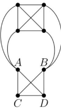
Proof. Consider first the first operation. It could result in a new K4 only if G contains the graph in Figure 3 as a subgraph. Since n > 13, each of the two Hamiltonian cycles whose union is G must reach this subgraph from the rest of the graph via C or D, and leave it from the other vertex in this pair. Thus neither cycle can contain the edge CD, a contradiction.
A B
C D
Figure 3. Impossible at the first replacement.
Suppose, for contradiction, that in the chain of operations a new K4 is generated. As before, the graph obtained so far necessarily is as in Figure 3. Since such a subgraph cannot be present in G, some edges have to come from previous operations on small archipelagos. Observe that each such operaton reduces the degrees of the vertices of the newly added edge. Thus the only edge in Figure 3 that could come from a previous deletion is the edge connecting C to D. In this case, before that deletion our graph had to look like in figure 4.
But in this case every vertex has degree four, thus G consists of just these 12 vertices,
contradicting our assumption that n >13.
7
A B
C D
Figure 4. Impossible, unlessn = 12.
Claim 3.12. Each operation results in a two-miltonian graph.
Proof. By induction on the number of operations. Assuming that after a deletion the resulting graph is the union of two Hamiltonian cycles H1 and H2, replace in each of H1, H2 the detour through the archipelago by the newly added edge.
This concludes Step 1. The resulting graph G1 is two-miltonian by Claim 3.12, and it contains no acyclic archipelagos with independent neighborhoods of size two. Note also that G1 is a supergraph of G′, and hence it is enough to prove Lemma 1.7 with G1
replacing G.
Step 2. Taking care of connectedness.
In this step we add edges, so as to make the graph G1 connected. These edges will remain in the next steps, and so we shall not have to worry about connectedness from this point on.
LetH1 be one of the two Hamiltonian cycles formingG1. LetG′1 be the graph obtained from G1 by removing all K4s from it, and let C1, . . . , Cm be the connected components of G′1. Define an auxiliary graphA on the vertex set V(A) :={C1, . . . , Cm}, two vertices Ci and Cj being connected if there is a path contained in H1, whose one endpoint is in Ci and the other in Cj and all the other vertices lie in a single archipelago. Since H1 is Hamiltonian, the graphAis connected. Choose a spanning tree ofA, and letP1, . . . , Pm−1
be subpaths ofH1 associated with each edge of the spanning tree. For each pathPi going through an archipelago Ki connect the endpoints of Pi in the graph G1, and delete all vertices of the archipelago Ki. The graphG2 obtained this way is connected, it does not contain any new K4s and ∆(G2)≤4.
Remark 3.13. If G′1 was not connected then the degree of some vertices decreases. This is true since removing an archipelago reduces the total degree of the vertices adjacent to it by at least 4, and the addition of an edge increases it only by 2.
The construction also yields:
Remark 3.14. Edges added in this process do not belong to a cycle in G2
Claim 3.15. Let K be an acyclic archipelago in a graph of maximum degree at most four. Suppose that the neighborhood N(K) is independent and has size 4 or more. Then
8
we can delete K and connect two vertices in N(K) by an edge, so that the new edge doesn’t generate a new K4.
Proof. Assuming negation, for every pair p = {x, y} of vertices in N(K)\V(K) there exists a pair q(p) ={u, v} ⊆V(G)\N(K) such that all pairs among x, y, u, vapart from xy are edges in G. We say that q(p) is a complementary pair of p.
Suppose first that there exist two pairs p1, p2 such that q(p1) 6= q(p2). If p1 ∩p2 = ∅ let p3 be a pair meeting both. Then q(p3) 6= q(pi) for i = 1 or i = 2 (or both), proving that there exist non-disjoint pairs p, p′ with q(p) 6=q(p′). Letv∗ be the vertex in p∩p′. If q(p)∩q(p′) = ∅ , then v∗ is connected to the four vertices in q(p)∪q(p′), and since as a member of I it is also connected to a vertex in K, its degree in G is at least 5, a contradiction. On the other hand, if there exists a vertex v∗∗ ∈ q(p)∩q(p′), then v∗∗ is connected to the five vertices in q(p)∪q(p′)∪p∪p′\ {v∗∗}, again a contradiction.
Remark 3.16. The proof yields a stronger result: it suffices to assume that in the indepen- dent neighborhood of the acyclic archipelago not all pairs have the same complementary pair.
Step 3. Deleting acyclic archipelagos with independent neighborhoods of size 3.
Let K be an acyclic archipelago such that N(K) is independent and has size 3, say N(K) = {A, B, C}. By Remark 3.16 if no pair in N(K) can be connected without generating a K4, all pairs must have the same complementary pair, and thusA, B, C are all connected to two vertices, O1 and O2. In such a case we call K forbidden and the 5-vertex subgraph showing this forbidding for K.
A B C
O1 O2
A forbidding subgraph
A′ B′ C′
O′1 O2′ Type 1
A′ B′ C′
O1′ O′2 Type 2
A′ B′ C′
O′1 O2′ Type 3 Figure 5. The forbidden subgraphK is invisible in the picture. The Type 1,2,3risking subgraphs are the three graphs (up to isomorphism) that are one edge short to be forbidding.
Claim 3.17. G2 does not contain a forbidden archipelago.
Proof. Suppose that G2 contains a forbidden archipelago with forbidding subgraph F, with vertices denoted as in the figure. Since A, B, C ∈ N(K), they do not belong to any archipelago J, or else K and J, being connected, would be contained in the same archipelago. The same is true forO1, O2, since they are of degree 4 in F. By Remark 3.14 no edges in F were added in Step 2. Also, no edges inside F was added in Step 3, since the endpoints of any edge that is added in Step 3 have maximum degree three. Thus F is also a subgraph of G. The archipelagoK consists of at most two K4s, since otherwise the degrees of some of the A, B, C would be larger than four. But then the subgraph consisting of the union of K and the verticesA, B, C, O1, O2 has at most 13 vertices, and it is connected to the rest of the graph by at most two edges. Since the endpoints of these two edges have degree 4, this contradicts the fact that G is two-miltonian on more than
13 vertices.
9
We next delete archipelagos one by one, taking care not to generate a forbidden archipelago. The risk is that connecting two neighbors of a deleted archipelago may create a forbidding subgraph for some other archipelago. Up to isomorphism, there are three subgraphs that are one edge short of the forbidding subgraph, see the graphs named Type 1,2,3 in Figure 5 (a step that helps in realizing this is noting that in the forbid- ding subgraph the role of O1, O2 and B, C is symmetric). We will say that an acyclic archipelagoK′ is riskyif it has an independent neighborhood consisting of three vertices that are connected, besides to vertices in K′, to vertices O1, O2, forming a graph Y of one of these three types. We say that the subgraph Y is risking for K. By Claim 3.5 K sends at least four edges to its neighborhood, and hence at least one of the vertices A, B, C receives from K two edges. As in the figure, we denote this vertex by A, and whenever “A” is used in this context we assume that it has degree at least 2 to the risky archipelago.
Claim 3.18. Let K′ be a risky archipelago contained in G2, and denote the vertices in its risking subgraph as in Figure 5. Then deleting K′ and connecting A′ to B′ does not generate a forbidding subgraph for some other archipelago.
Proof. LetY be the risking subgraph of K′. Suppose, by negation, that deleting K′ and adding the edge e = A′B′ generates a forbidden archipelago K. This was born from a risking graph Z forK. Denote the vertices ofZ by A, B, C, O1, O2, as in the figure. Since at least two edges were removed from the star of A′ and only one edge was added, the degree ofA′ strictly decreases by the operation. If Z is of type 1, then the edge added is betweenO1 and O2, both of which become of degree 4, and thus the one that is identical toA′ had degree at least 5 before the operation. This is impossible, since throughout the process degrees of vertices do not increase, and ∆(G)≤4. A similar argument applies if Z is of type 3, and the added edge is AO1. Thus we may assume that Z is of type 2, and that e=B′O′1, see Figure 6.
Since the degree ofA′ decreased, and after the addition ofethe vertexO′1has degree 4, it is impossible thatA′ =O1′. Hence A′ =B and B′ =O1, see Figure 6. IfY is of Type 1 or 2, thenA′ is connected to the two opponents which are not inside any archipelago. But A′ has already 3 different neighbors in archipelagos (two from Y and at least one from Z), implying that A′ has degree at least 5 in G, a contradiction. Thus we may assume that Y is of type 3.
A B C
O1 O2
A′
=
B=′ =O2′
Figure 6. C′ can not be any vertex in this picture, and it must also be connected toO′2, a contradiction.
Since in a Type 3 subgraph,A′ is connected toO′2, we conclude thatO2 =O2′ or elseA′ would have degree 5. Since A′, B′, C′ are independent,C′ must be a vertex different from A, B, C, O1, O2, and since in a Type 3 subgraph C′ is connected to O2′ which is equal to O2, this means thatO2 has degree 5, again a contradiction.
10
By the claim it is possible to delete all risky acyclic archipelagos one by one,
We now remove acyclic archipelagos with neighborhoods of size 3, adding an edge at each stage, as follows. If at the current stage there are no risky acyclic archipelagos we delete any archipelago with independent neighborhood of size 3 and connect two of its neighbors, without risking the generation of a K4 (since there are no forbidden archipelagos), and without generating a forbidden archipelago (since there are no risky archipelagos). At stages in which there is a risky archipelago we use the claim to remove such an archipelago, while not generating a risky archipelago, and not generating a K4
(the latter following from the non-existence of a forbidden archipelago).
LetG3 be the graph obtained after these operations. ThenG3 is connected, it does not contain any new K4s, and ∆(G3)≤4.
Step 4. Removing all remaining archipelagos.
Since G3 does not contain any acyclic archipelagos with independent neighborhoods of size two or three, by Lemma 3.15 we can delete every acyclic archipelago with an independent neighborhood one by one, and after each deletion we can connect some vertices in their neighborhood without creating a newK4. After we deleted every acyclic archipelago with an independent neighborhood, we delete every other acyclic archipelago and every other cyclic archipelago without adding any additional edges. Let H be the graph obtained fromG3 this way.
We claim thatH satisfies the requirements of the lemma. Clearly, it isK4-free, and Step 2 saw to it that it is connected. At each step of our construction degrees of vertices only went down. If in Steps 1 or 3 any archipelagos were deleted, the degree of some vertices strictly decreased, since only one edge is added, while at least 4 edges were removed as the result of the removal of the archipelago. By Remark 3.13 each deletion of archipelagos in Step 2 also decreased the degree of at least one vertex. Condition 4 in the lemma follows
from our construction and Claim 3.7.
Remark 3.19. The two-miltonian property of G was used:
• For the property that ∆(G)≤4 .
• For the property that theK4s in Gare vertex disjoint.
• For the property that an acyclic archipelago sends a certain number of edges to its neighbourhood. This can be avoided since if it would send less, we could treat it as if it is a cyclic archipelago.
• In Step 1 to forbid subgraphs like in figure 3. This is important since we have to forbid graphs like 1 as Lemma 1.7 can not be applied to such graphs.
• In Step 2 to guarantee connectedness. This could be avoided by paying attention to the connectedness of the K4-free part at each deletion. (Although this would make the proof even more unpleasant to read.)
Thus the authors feel that results similar to Lemma 1.7 should hold with assumptions on Gthat can replace the role of two-miltonicity at the above mentioned parts of the proof.
Corollary 3.20. In a two-miltonian graph G on n vertices
α(G)≥ζ(G) + 7
26(n−4ζ(G))−O(1).
Proof. LetH be the graph obtained from Gas in Lemma 1.7. By Theorem 1.5 α(H)≥
7
26|V(H)| −O(1) = 267 (n−4ζ(G))−O(1), and by part (4) in the conclusion of the lemma
α(G)≥α(H) +ζ(G).
11
4. Calculating f(n, n/4)
We will use a theorem that was proved by Albertson, Bollob´as and Tucker. We state it in a simplified form, tailored to our needs. For the more general version see [1]
Theorem 4.1 (M. Albertson, B. Bollob´as, S. Tucker). If G isK4-free, ∆(G)≤4and G is not 4-regular, then α(G)> n4.
The value off(n, n/4) can be determined for all n.
Theorem 4.2.
(1) If 4∤n thenf(n, n/4) = 1.
(2) f(4,1) =f(8,2) = 3.
(3) f(4k, k) = 2 for k≥3.
Proof. Part (1) follows from Brooks’ theorem. The following figure shows that for every k there exists a two-miltonian graph G with n = 4k and α(G) =ζ(G) = k. This means that f(4k, k)≥2.
Figure 7. The two strips eventually close on themselves.
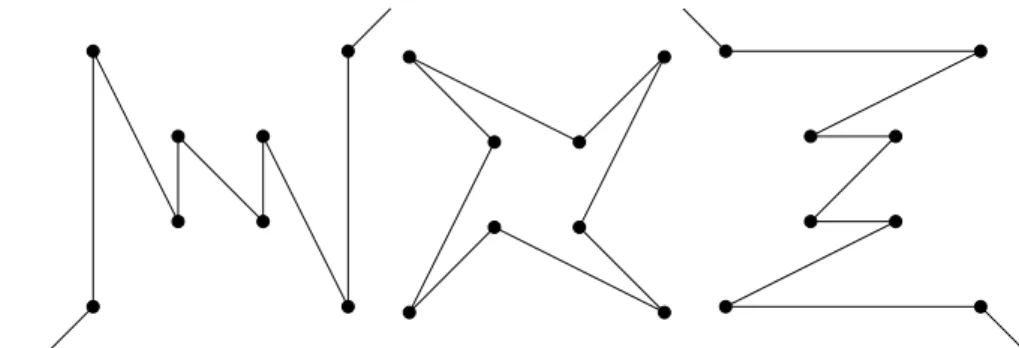
Since there are only three distinct Hamiltonian cycles on 4 vertices, the fact that f(4,1) = 3 is easy. Figure 8 is an example of three Hamiltonian cycles on the same vertex set of size 8, having each pairwise union K4 -covered, thus α(Ci ∪Cj) = 2 for 1≤i < j ≤3, showing thatf(8,2)≥3.
Figure 8. The vertices are identified by horizontal shifting, showing that f(8,2)≥3
Each pair of dangling edges in the two extreme cycles are meant to join to form one edge. For our next arguments we will need the following lemma.
Lemma 4.3. If 4 | n and n ≥ 12 then there do not exist three Hamiltonian cycles C1, C2, C3 such that Ci∪Cj isK4-covered for all pairs1≤i < j ≤3.
Proof. Assume for contradiction that we do have three such cycles. Enumerate the vertices 1, . . . ,12 so that i(i+ 1)∈ E(C1) for all i ≤ 12 (cyclical counting), and 1,2,3,4 form a K4 inC1∪C2. Then the edges ofC2 inside the three K4s formingC1∪C2 must be as in Figure 9.
12
1 2 3 4 5 6 7 8 9 10 11 12 Figure 9. The edges of C2 that form the K4s in C1 ∪C2 on the twelve vertices that we focus on.
Degree considerations and the fact that C2 is Hamiltonian yield that it is necessarily edge disjoint from C1. In general, all three cycles are edge disjoint.
Since C1∪C3 is also K4-covered, we can also draw the edges of C3 that form the K4s inC1∪C3 on the same vertex set:{1, . . . ,12}. This must be very similar to Figure 9, but it might be shifted as we cannot assume that the vertices 1,2,3,4 form a K4 inC1∪C3. Moreover, since we already know that the cycles are edge disjoint, it should be shifted by exactly two vertices. Figure 10 describes the union of the edges of C2 and C3 that form the K4s in their union with C1. This is also a subgraph ofC2∪C3.
1
2 3
4 5
6 7
8 9
10 11 12
Figure 10. A subgraph of C2∪C3.
The edges in Figure 10 form a 3-regular subgraph of C2 ∪C3, thus every vertex has an additional neighbor (since C2 is edge disjoint from C3). Observe that if the vertices labeled 5,6,9 form an independent set, their neighborhood is of size at most 9 inC2∪C3
and by Observation 3.6 we can enlarge it to an independent set of size more than n/4 in C2∪C3, a contradiction. Thus there must be an edge connecting some of the vertices labeled 5,6,9. In Figure 10 the vertices 5,9 already have two edges from C2, and the vertex 6 has two edges from C3, so no edge can connect 6 to 5 or 9. Thus 5 and 9 must be connected (by an edge in C3). But then by shifting the whole argument to the left by four, we get that 1 should be also connected to 5 in C3, which contradicts the fact that
C3 is a cycle.
The proof that f(8,2) ≤ 3 and f(12,3) ≤ 2 can be done by computer. It remains to be shown that f(n, n/4) ≤ 2 when n is divisible by four and n ≥ 16. Assume for contradiction that f(n, n/4)≥3 thus there exist three Hamiltonian cycles C1, C2, C3 on n = 4k vertices, such that α(Ci∪Cj) = n4 whenever 1 ≤ i < j ≤ 3. Then each union Ci∪Cj contains a copy ofK4, since otherwise by Theorem 1.5 there exists an independent set of size (7n−4)/26, which is strictly larger than n/4 whenn ≥16. We next show that Ci∪Cj not only contains a single K4, but it isK4-covered. Assuming that this is not the case, since there is at least one K4 inG, by Lemma 1.7 there exists a K4-free nonempty subgraph H that has at least one vertex of degree at most three. But then Theorem 4.1 yields an independent set in H strictly larger than|V(H)|/4, and by Lemma 1.7 we can enlarge it to an independent set of size more than n/4 in Ci∪Cj. Thus Ci∪Cj must be K4-covered, but this contradicts Lemma 4.3 and the proof is complete.
Remark 4.4. Supopse that we are interested in the maximal number of Hamiltonian paths (instead of Hamiltonian cycles) with the property that the union of any two has independence number at most n/4. It can be proven that when n is divisible by four we can have at most two Hamiltonian paths (and we can have two, see Figure 7 without the strips closing on themselves) and otherwise we can only have a single one by the
13
usual Brooks reasoning. In this context, n = 8,12 are exceptional only because we are interested in Hamiltonian cycles instead of paths.
5. A lower bound on ct
We will use the following observation.
Claim 5.1. [4] Let y be a vertex of G with exactly two neighbors x and z such that x and z are not connected. Let G′ be a graph defined by V(G′) = V(G)\ {x, y, z} ∪ {v}
where v is a new vertex connected to all remaining neighbors of x and z. Thus deg(v) = deg(x)+deg(z)−2. Then for any independent setI′ ofG′, we can construct an independent set I of G of such that |I|=|I′|+ 1.
Proof. Ifv ∈I′ thenI =I′ \ {v} ∪ {x, z}. If v /∈I′ then I =I′∪ {y}.
Notation 5.2. We call a subgraph ofG good if it is an induced path of length three We write ψ(G) for the maximal number of vertex disjoint good subgraphs inG.
In a two-miltonian graph all copies of K4 are vertex disjoint, so ζ is the number of disjoint copies of K4.
Observation 5.3. Let C, D1, D2 be Hamiltonian cycles, and let m be the number of K4s that are contained in both C∪D1 and C∪D2. Then ψ(D1∪D2)≥m.
Proof. In every K4 contained in both C∪D1 and C∪D2 the edges that do not belong
toC form a path of length 3 in both D1 and D2.
Lemma 5.4. If G is 2-miltonian then α(G)≥ 7
26n− 1 13ζ+ 1
2ψ −O(1) Proof. Lete=|E(G)|. By Theorem 3.1 e−9n+ 26α(G)≥ −4.
Let G1 := C1 ∪ C2. Let T be a set of disjoint good subgraphs of size ψ. For each path Pi ∈ T, using the notation of Figure 11 below, we apply the operation described in Claim 5.1, of removing x, y, z and adding a vertex v =vi connected to the remaining neighbors of x, z. Let G2 be the graph obtained by combining all these ψ operations.
Then |V(G2)|=n−2ψ.
x y z
Figure 11. A good subgraph in C1∪C2.
Observe that G2 is still two-miltonian and that ζ(G2) = ζ(G). Let H be the graph obtained from G2 using Lemma 1.7. ThenH is a subgraph of G2, it is simple, connected, and K4-free. We have |V(H)|=n−4ζ−2ψ, and since every vertex vi, and its unnamed neighbor in Figure 11 has degree at most 3 in H, we have
2|E(H)| ≤4((n−4ζ−2ψ)−2ψ) + 6ψ = 4n−16ζ−10ψ.
Thus using the inequality in the second remark of Theorem 3.1 we get that α(H)≥ 9|V(H)| − |E(H)| −4
26 ≥ 9(n−4ζ−2ψ)−(2n−8ζ−5φ)
26 − 4
26 =
14
= 7
26n− 28
26ζ −13
26ψ−O(1) = 7
26n− 14 13ζ− 1
2ψ−O(1).
By Lemma 1.7 we can enlarge this independent set to an independent set of G2 of size α(G2)≥ 7
26n− 1 13ζ− 1
2ψ−O(1).
By Claim 5.1 we have an independent set in G1 of size α(G1)≥ 7
26n− 1 13ζ+1
2ψ−O(1)
finishing the proof.
Lemma 5.5. Let ε > 0 be fixed and S = {S1, . . . , Sm} be a set system on a ground set of size n with the following properties.
• ∀i: |Si| ≥xn
• ∀i6=j : (1−ε)x2n ≥ |Si∩Sj|
Then m is bounded by a number independent of n:
m≤q(x, ε) = 1−x(1−ε) xε .
Proof. Letz =xm. LetX1 andX2 be two uniformly randomly and independently chosen sets from S. Let us denote by li the number of sets in S which contain the element i.
Now we have that:
E(|X1∩X2|) =
n
X
i=1
P(i∈X1∩X2) =
n
X
i=1 li
2
m 2
Since the average of the li is exactly z, and the function x(x−1)2 is convex, by Jensen’s inequality we have the following
n
X
i=1 li
2
m 2
≥n
z 2
m 2
=n z(z−1)
z x
z
x −1 =n z−1
z
x2 − 1x =nx2z−1 z−x. Elementary calculation yields that the inequality
z−1
z−x ≤(1−ε)
holds if and only if m= zx ≤ 1−x(1−ε)xε , finishing the proof.
Remark 5.6. If in Lemma 5.5 we replace (1−ε)x2n by (1 +ε)x2n, we can construct set systems of exponential size by a uniform random construction.
For 0< x≤1 and ε >0 let δ(x, ε) =
qx 4, ε
+ 1−1
=
4−x(1−ε) xε + 1
−1
.
Lemma 5.7. For every 0 < x ≤ 1 and ε > 0 there exists a number θ(x, ε) such that if k > θ(x, ε) and X = {C1, . . . , Ck} is a collection of Hamiltonian cycles satisfying
xn
4 ≤ζ(Ci∪Cj) whenever 1≤ i < j≤k then there exists a subcollection X2 ⊆X of size at least |X|δ(x,ε), such that (1−ε)x162n ≤ψ(Ck∪Cl)for every pair of cycles Ck, Cl ∈X2.
15
Proof. LetA be a graph whose vertex set is X, and two cycles Ci and Cj are connected by an edge if and only if (1−ε)x162n ≤ψ(Ci∪Cj). Our aim is to show that|X|δ(x,ε) ≤ω(A) (the latter denoting the largest size of a clique in A). This will follow from Ramsey’s theorem and an upper bound we shall obtain on α(A).
Claim 5.8. α(A)≤q(x4, ε) + 1 = 4−x(1−ε)xε + 1.
Proof. Suppose to the contrary that there exists an independent set D1, D2, . . . Dp in A, where p = ⌈q(x4, ε)⌉+ 2. By relabeling the vertices, we can assume that D1 is the cycle (1,2, . . . , n). For every 1< j ≤p let Sj be the set of those 1≤i ≤n for which D1∪Dj
contains a K4 on the vertices i, i+ 1, i+ 2, i+ 3(modn).
By the assumption of the lemma ζ(D1∪Dj) ≥ xn4 , and hence |Sj| ≥ xn4 for all j ≤p.
Since the cycles Dj are independent in A, ψ(Di ∪ Dj) < (1−ε)x16 2 whenever i 6= j. By Observation 5.3 this implies that|Si∩Sj|< (1−ε)x16 2n.
These combined yield a contradiction to Lemma 5.5.
By a result of Ajtai, Komlos and Szemeredi [3], for fixed sand t large enough we have the following bound on the Ramsey numbers:
R(s, t)≤cs
ts−1 log(t)s−2,
implyingR(s, t)≤ts for fixeds and large enough t. Thus for fixed s and large enough n if G is a graph on n vertices with α(G) ≤ s then ω(G) ≥ n1s. Applying this to the graph A, and using Claim 5.8, we obtain that ω(A)≥ |X|(q(x4,ε)+1)−1 =|X|δ(x,ε) and the
proof is complete.
For a family X of Hamiltonian cycles let m(X) = minC6=D∈X ζ(C∪D)
n ∈ [0,1]. For the sake of readability, we will often write m for m(X).
Lemma 5.9. Let X be a set of Hamiltonian cycles, if ψ(C∪D)n < (1−ε)
ζ(C∪D) n
2
−ε for every pair C 6= D of cycles in X then there exists a subset Y of X of size at least
|X|δ(4m,ε) such that
m(Y)2 > m(X)2+ ε (1−ε).
Proof. By Lemma 5.4 and the fact that d is positive m > 0. Applying Lemma 5.7 with x = 4m, we obtain Y ⊆ X of size at least |X|δ(4m,ε), such that every pair of cycles C, D ∈ Y satisfies ψ(C∪D)n ≥ (1−ε)m2. Let C, D ∈ Y be such that ζ(C∪D)n = m(Y). By the assumption of the lemma
(1−ε)m(Y)2−ε= (1−ε)
ζ(C∪D) n
2
−ε > ψ(C∪D)
n ≥(1−ε)m2, which yields the desired result.
Corollary 5.10. If X is a set of Hamiltonian cycles satisfying
|X|
δ(4m,ε)1−εε
> θ(m, ε) then there exists a pair C 6=D of cycles in X such that
ψ(C∪D)
n ≥(1−ε)
ζ(C∪D) n
2
−ε.
16
Proof. Assume negation. Applying Lemma 5.9 repeatedly, we obtain then a sequenceX = X1 ⊇X2 ⊇. . .⊇Xp of sets of Hamiltonian cycles, such thatm(Xi+1)2 ≥m(Xi)2+(1−ε)ε and |Xi+1| ≥ |X|δ(4m(Xi),ε) for all i < p. Since δ(x, ε) is increasing in x and the sequence m(Xi) is increasing, the assumption on the size ofX thus leads to the conclusion that for pas large as 1−εε + 1 we still haveXp 6=∅. But this yieldsm(Xp)>1, which is impossible
since by definition m ∈[0,1].
We can now obtain our goal - a lower bound on the threshold constant ct. Remember thatct is a real number such that forc < ctthe value of f(n, cn) is bounded by a constant independently of n, and for c > cn this value is exponential in n.
Theorem 5.11. ct≥ 16945 ≈0.26627.
Proof. Letε >0 be fixed, and let d be positive such thatct< 267 −d. Let n be large and X be a large collection of Hamiltonian cycles onnvertices such that for every pairC 6=D of cycles inX we have α(C∪D)≤(267 −d)n. Here “large” is dictated by Corollary 5.10
By Corollary 5.10 there exist cyclesC 6=D∈Xfor which ψ(C∪D)n ≥(1−ε)
ζ(C∪D) n
2
− ε. By Lemma 5.4
7 26−d
n≥α(C∪D)≥ 7
26n− 1
13ζ(C∪D) + 1
2ψ(C∪D)−O(1) and thus
−d≥ − 1 13
ζ(C∪D) n + 1
2
ψ(C∪D)
n − O(1) n
−d≥ − 1 13
ζ(C∪D) n + 1
2((1 +ε)
ζ(C∪D) n
2
−ε)−O(1) Since we can choosen arbitrarily large andε arbitrarily small, it follows that
−d≥ − 1 13
ζ(C∪D) n + 1
2
ζ(C∪D) n
2
by taking the minimum of the right hand side we get that d≤ 1
338 ≈0.002958
for every choice of d where 267 −d > ct, thus ct≥ 267 − 3381 = 16945 ≈0.266272
References
[1] M. Albertson, B. Bollob´as, and S. Tucker,The independence ratio and maximum degree of a graph, Congressus Numerantium (1976).
[2] N. Alon and J. H. Spencer,The probabilistic method - Fourth edition, Wiley, Tel-Aviv, 2016.
[3] M. Ajtai, J. Komlos, and E. Szemeredi,A note on Ramsey numbers, J. Combin. Theory Ser. A 29 (1980), 354-360.
[4] E. Cs´oka, Independent sets and cuts in large-girth regular graphs, arXiv:1602.02747 [math.CO]
(2016).
[5] S. Janson, T. Luczak, and A. Rucinski,Random graphs, Wiley, New York, 2000.
[6] S. C. Locke and F. Lou, Finding independent sets inK4-free 4-regular connected graphs, Journal of combinatorial theory, Series B71(1997), 85-110.
[7] L. Lov´asz,A note on Ramsey numbers, J. Combin. Theory Ser. A25(1978), 319-324.
[8] A. Schrijver,Vertex-critical subgraphs of Kneser graphs, Nieuw Arch. Wiskd.26(1978), 454?461.
17
Department of Mathematics, Technion, Haifa, Israel E-mail address, Ron Aharoni:raharoni@gmail.com
Department of Computer Science and Information Theory, Budapest University of Technology and Economics
E-mail address, Daniel Solt´esz:solteszd@math.bme.hu
18


![arXiv:2002.11678v2 [math.FA] 11 Sep 2020](data:image/gif;base64,R0lGODlhAQABAIAAAP///wAAACH5BAEAAAAALAAAAAABAAEAAAICRAEAOw==)