BUDAPEST WORKING PAPERS ON THE LABOUR MARKET
BWP – 2018/3
Demand for secondary school characteristics Evidence from school choice data in Hungary
THOMAS WOUTERS - ZOLTÁN HERMANN - CARLA HAELERMANS
BWP 2018/3
INSTITUTE OF ECONOMICS, CENTRE FOR ECONOMIC AND REGIONAL STUDIES HUNGARIAN ACADEMY OF SCIENCES
BUDAPEST, 2018
2
Budapest Working Papers on the Labour Market BWP – 2018/3
Institute of Economics, Centre for Economic and Regional Studies, Hungarian Academy of Sciences
Demand for secondary school characteristics Evidence from school choice data in Hungary
Authors:
Thomas Wouters KU Leuven
email: thomas.wouters@kuleuven.be Zoltán Hermann
research fellow
Institute of Economics, Centre for Economic and Regional Studies, Hungarian Academy of Sciences, Hungary (CERSHAS) and Corvinus University of Budapest
email: hermann.zoltan@krtk.mta.hu
Carla Haelermans associate professor Maastricht University
email: carla.haelermans@maastrichtuniversity.nl
June 2018
3
Demand for secondary school characteristics
Evidence from school choice data in Hungary
THOMAS WOUTERS - ZOLTÁN HERMANN - CARLA HAELERMANS
Abstract
We estimate preferences for school tracks in upper secondary education in Hungary.
We consider travel time, school SES composition, school level (in terms of peer quality) and school quality (in terms of added value). We find that students have stronger preferences for school SES composition and school level, rather than school quality (which may be harder to observe). Furthermore, these preferences vary between high- and low-ranked schools, indicating students use heuristics in the process of compiling their ranked preference list.
Keywords:school choice, school composition, school quality, rank-ordered logit
JEL: I21, I24
Acknowledgement:
The project leading to this application has received funding from the European Union's Horizon 2020 research and innovation programme under grant agreement No. 691676.
4
Iskolai jellemzők és a középiskolák iránti kereslet
Eredmények a magyarországi középiskolai jelentkezési adatok alapján
THOMAS WOUTERS - HERMANN ZOLTÁN - CARLA HAELERMANS
Összefoglaló
A tanulmány jelentkezők középiskolákra vonatkozó preferenciáit vizsgálja magyar adatok felhasználásával. Négy tényezőt vizsgálunk: az iskola utazási idővel mért távolságát, a diákok társadalmi háttér és korábbi tanulmányi eredmény szerinti összetételét, és az iskola hozzáadott- érték mutatóval mért minőségét. Az eredmények azt mutatják, hogy a jelentkezők sokkal inkább figyelembe veszik a diákok összetételét, mint az iskola minőségét, ami közvetlenül nehezen megfigyelhető. Ugyanakkor eltérő szempontok érvényesülnek az első jelentkezések és a kevésbé preferált iskolák kiválasztásakor.
JEL: I21, I24
Tárgyszavak: iskolaválasztás, diákok összetétele. Iskolaminőség, rangsor-logit
5 0. INTRODUCTION
Many countries have a system of school choice, where parental and/or student preferences play a role in school assignment. Choice may be restricted in several ways. Schools can impose minimum entry grades, or may have preferences for a diverse student body (controlled school choice). What factors drive students’ choice behavior is of high relevance for the effects that can be expected from introducing a school choice system.
It is argued that school choice should increase school quality, as long as students and their parents are rational decision makers who maximize their utility by choosing the best school possible. Many studies have shown that school quality indeed is one of the determinants of school choice, and other studies in turn have shown that increased school choice indeed has led to higher school quality, mostly through increased competition (see e.g. Burgess et al., 2014), as schools will have to increase their quality in order to attract enough students to be feasible.
However, if the effect of quality is weak, there is no incentive for the school to compete on quality, and therefore other factors, such as profile and educational philosophy of the school come into play.
This can also be seen from the literature, where it is shown that other factors (such as distance, SES (socio economic status) or ethnic composition, religion, teachers, profile and educational philosophy of the school) also play an important role in school choice. And it is shown that school choice does not only lead to higher school quality, but also to higher segregation (see e.g. Lankford and Wyckoff, 1992; Denessen et al., 2005; Borghans et al., 2014).
So school choice can also have detrimental effects on equality of opportunity, when disadvantaged students end up in lower quality schools.
However, previous literature is in most cases based on observed choices, rather than observed preference lists. The downside of using observed choices rather than an overview of preferences is that it is harder to determine which characteristics have made the differences in the school choice. Preference list allow to rank the characteristics of a school and determine the order of importance. Only few studies actually use listed preferences (e.g. Burgess et al., 2014).
Furthermore, most studies on the determinants of school choice concern primary education, and thereby parental choices. Furthermore, only a few studies consider secondary education, where students’ preferences matter to a larger degree in the school choice process (examples are Müller et al., 2008, Burgess and Briggs, 2010, Chumacero et al., 2011, Karsten et al., 2003 and Ruijs and Oosterbeek, 2014).
6
In this paper, we estimate the determinants of preferences for upper secondary schools, using a dataset on school choice in Hungary. We study whether school quality (measured both as the absolute level of student performance prior to secondary education (so student quality, or selection) as well as learning gains between primary and secondary school) and school SES composition affect students’ choices, controlling for actual travel time data from home to school.
We focus on what is more important in school choice: the level of the school, or school quality (measured as learning gains). We use data from listed preferences for schools and school tracks, for over 4 million students entering upper secondary education from one single cohort. The data include the school/track characteristics mentioned before, as well as background characteristics of the students. We use a ranked-ordered logit model to estimate preferences for school choice.
In doing so, the contribution of our paper is threefold:
1) We use the actually listed school preferences per student, contrary to most studies that use realised school choice decisions.
2) We use a ranked-ordered logit model, such that we are not constrained to studying how students decide on their highest-ranked school. We also use information on the ranking of schools further down the preference list.
3) We study secondary school choice, a more high-stakes decision than primary school choice.
In the remainder of this paper, we proceed as follows: We first describe the relevant literature on school choice, before we discuss Hungarian secondary education and the school choice system in Hungary. Then, the data and ranked-ordered logit model that we use for our analysis are presented. Section 5 shows the results, in which we discuss the baseline model, and the results by track, followed by an analysis of how students construct their choice set. Lastly, section 6 presents the conclusion and discussion.
1. LITERATURE REVIEW
The literature on school choice can roughly be divided into two strands. The first one studies the determinants of school choice, whereas the second one provides evidence on the effects of school choice on performance and other outcomes. In this paper, our focus lies on the first part, the determinants of school choice. We can infer several student and school characteristics from the literature that are relevant for the school choice process. The three most commonly found determinants are 1) school quality, measured as student performance (Lankford and Wyckoff,
7
1992; Black, 1999; Alderman et al., 2001; Denessen et al., 2005; Hastings et al., 2008, Dronkers and Avram, 2010; Chumacero et al., 2011; Koning and van der Wiel, 2013; Borghans et al., 2014;
Burgess et al., 2014; Cornelisz, 2014), 2) the distance between home and school (Glazerman, 1998; Elacqua et al., 2006; Hastings et al., 2008; Müller et al., 2008; Burgess et al., 2011;
Chumacero et al., 2011; Borghans et al., 2014; Burgess et al., 2014), and 3) the share of students with another ethnicity, race or SES (Socio Economic Status) at the new school (Lankford and Wyckoff, 1992; Glazerman, 1998; Burgess and Briggs, 2010; Dronkers and Avram, 2010; Burgess et al., 2014; Cornelisz, 2014).
Other, less frequently mentioned determinants are religion (Lankford and Wyckoff, 1992;
Denessen et al., 2005; Borghans et al., 2014), the teachers (Jacob and Lefgren, 2007), information provision, on either school quality (Hastings et al., 2007; Hastings & Weinstein, 2008; Koning and van der Wiel, 2013; Allen and Burgess, 2013), or on the odds of admission (Hastings et al., 2007), the specific profile of the school, for example a language profile (Müller et al., 2008), or the educational philosophy (Borghans et al., 2014).
However, preferences for school choice may differ by the background of the student (or parents) making the school choice (or the decision to move to a certain catchment area).
Hastings et al. (2005), for example, show that parents with higher income and higher academic ability have a stronger preference for school test scores. This is confirmed by Burgess et al.
(2014), who show that more advantaged parents have a stronger preference for academic performance. Burgess et al. (2009) show that the more educated parents, as well as higher SES parents, have a stronger preference for school quality and school social composition, whereas the less educated and lower SES have a stronger preference for proximity. In line with this, Burgess and Briggs (2010) find that children from poor families are less likely to attend good schools.
This is mostly, but not completely, due to location. Dronkers and Avram (2010) also show that upwardly mobile parents have a stronger preference for better performing schools, however, they also show that lower and middle class parents have a stronger preference for segregation.
Besides differences in student background, there are also quality difference in these studies, as some of them provide pure descriptives and correlations (e.g. Karsten et al., 2003; Denessen et al., 2005; Burgess et al., 2011), whereas other studies use more (quasi-) experimental approaches, or mixed logit models that are more flexible regarding the IIA property. Examples of the latter are Borghans et al., (2014), Burgess et al. (2014) and Hastings et al. (2005).
There are a few studies described above that resemble our study, as they also have explicit rankings of students (and not only observed school choice). These are Burgess et al. (2014), using a conditional logit model and Hastings et al. (2005), using a mixed-logit demand model.
8
However, both these studies take place in primary education, whereas the study at hand focuses on secondary education.
2. INSTITUTIONAL CONTEXT
Compulsory education in Hungary is organised in a two-tier system. General schools, covering grade 1-8 provide primary and lower-secondary level education. After completing the general school students apply to upper-secondary schools. At this stage, students choose from a diverse supply of educational programs. Due to differences in school quality and specialisation, this choice has long-lasting effects on the educational and professional career of students.
Upper-secondary education in Hungary follows three tracks. In the academic track (gymnasium) students prepare to enter higher education. Some schools also offer longer academic secondary studies starting in grade 5 or 7 instead of grade 9. These are the most selective studies, covering 6-8% of the students. In this paper we focus on the choice after grade 8, and the latter group of students are not included in our analysis. The vocational secondary or mixed track also enables students for higher education, but the curricula are less academically oriented and include preparatory courses for vocational training as well. However, at the end of grade 12 students of both tracks take the same final exam, also serving as an entrance exam to higher education. Vocational training in the mixed track is provided in a separate program, starting in grade 13. The third track is the vocational school which provides a lower level vocational qualification. The study length in this track is four years as well, but grade 11 and 12 cover vocational training. Students from this track are not qualified to apply to higher education programs. There are marked differences in the prestige of the three tracks. Students and parents almost exclusively rate the academic track higher than the mixed one, which they place above the vocational track. Overall the mixed track has the highest enrolment share, followed by the academic and the vocational track.
The application and admission to upper-secondary education are organised at the national level, built around a centralised matching scheme (see Bíró, 2012 for a detailed description).
Schools offer, and students apply to general or specialised studies. These often comprise of a single class within the school. An academic school, for example, may offer a general academic program, a class with advanced math and a class specialised in French. In the mixed and the vocational tracks, the programs are most often defined by the field of study. Schools set quota for each programme on offer. Students are free to apply to any school. They choose the educational programs they want to apply for, and submit a ranked list. It is important to note that the
9
matching scheme provides no incentive for strategic application, i.e. if a student prefers school A to B, she cannot obtain a better outcome by ranking B over A (Bíró, 2012). Next, schools decide which students they strictly reject and rank the accepted applicants. Schools rely on grades in general school, but may also require students to take a written entrance exam or an interview.
Schools may also consider other student characteristics, e.g. religious affiliation in church schools, or a sibling already enrolled in the school. There is considerable freedom to set and weight different admittance criteria. However, rankings are mostly built on some measure of prior student performance. Finally, students are allocated to schools by a Gale-Shaply algorithm, taking into account submitted student preferences, schools’ rankings of applicants and the available seats in the schools. Overall, the admission system generates a strict sorting of students across schools that is essentially merit-based. There is no incentive for students or schools to deviate from their true preferences. Nevertheless, students typically limit their application list to 3-10 programs. Students mostly ignore schools that are well beyond their reach regarding their level of achievement.
In Hungary, several schools provide education in two or even all three tracks, while others are specialised into education in one of the three tracks. Though students might prefer either more or less specialised schools for several reasons, we do not analyse this aspect directly. For the sake of simplicity we define schools providing education in a given track, i.e. we divide institutions with a broader profile into two or three separate schools. Henceforward in the paper, we use the term school in this sense.
A unique feature of the admission system in Hungary is that students apply to education programs within schools. These programs are often small, covering a single class of students or even half of a class. Due to the small number of students, school quality could be estimated at this level only with substantial error. In order to mitigate measurement error, we aggregate the application data to the school level. In case of students applying to more than one education program offered by the same school, we assign to this school the highest rank within the school.
E.g. if a student applies to school A at the first and third place, and lists school B at the second and fourth place, we consider school A as her first choice and school B as the second.
3. DATA AND METHOD
DATA
Our sample represents a single cohort of students who have completed grade 8 in 2006.
The sample was created by matching two administrative data sets, the 2006 wave of the National
10
Assessment of Basic Competences (NABC) and the Upper-Secondary Education Application and Admission register (USEAA). The NABC file includes math and reading literacy scores from low-stake standardised tests; grade point average attained in general school, and data on students’ family background, including parental education. The USEAA register contains detailed application data. We observe the full list of educational programmes and schools where the student applied to and the preference ranking submitted. Both datasets are intended to cover the full cohort. However, the NABC data do not include students who were absent on the day of the test, and family background variables are missing for the students who did not answer the background questionnaire. Finally, we merged travel time data to each student-school pair.
Travel time data comes from the GEO database of the Institute of Economics of Budapest.
Due to missing data and the imperfect matching of the two datasets our sample covers about three quarter of the 2006 cohort. Applications to distant schools with unreasonable travel time were also excluded. The final sample includes 69559 students, with 187216 applications to 1359 schools.
In the analysis we use two measures of student characteristics, prior achievement, measured by the mean of standardized math and reading test scores in grade 8, and parental education.
The latter is measured by a dummy variable indicating secondary level education, excluding the vocational track, or a higher education degree.
Our key variables are distance to school and school characteristics. We measure the distance to school by travel time in hours using public transport between the place of residence of the student (ZIP-code level) and the school.
We explore the effect of three school characteristics: school quality, socio-economic composition and the mean level of achievement.
ESTIMATING SCHOOL QUALITY
To measure school quality, we estimated the following student-level value-added model:
where A denotes grade 10 test score for student i in school j in year t, X and Z are vectors of student- and school-level controls respectively, π stands for year fixed effects and μ represent school effects. The student-level controls are third order polynomials of lagged scores, both math and reading, gender, special education needs status, mother’s and father’s education and the number of books at home.
11
School-level controls are the mean of lagged scores, both math and reading. In general, assessing school quality from the individual student’s point of view, student composition should not be controlled for (Raudenbush and Willms, 1995). Students can be assumed to take into account the expected outcome of enrolling in a given school, and do not care whether the gain is a result of peer effects or pure school quality (e.g. better teachers). However, as we are interested in comparing the effects of quality and student composition, we control for the latter, to remove the correlation between our quality and composition measures.
Following Kane and Staiger (2008) and Chetty et al. (2014), we model the school effects as random effects, with 0 mean and standard deviation of 1, and estimate the values of μ as an empirical Bayes residual or shrinkage estimate. This is the best linear estimator of μ, adjusting the initial school effects based on measurement error. The estimates are shrunk towards the overall mean of 0, with greater shrinkage for schools for whom fewer data are available. This way the estimation-error variance is reduced, which is important to mitigate attenuation bias in models including the estimated school effect as an explanatory variable (Koedel et al., 2015).
We estimate average school effects for the 2006-2010 period, assuming that school quality has not changed significantly over this short period. After estimating equation 1 for math and reading separately, we constructed a single quality measure by taking the average of the two and standardising it to have 0 mean and a standard deviation of 1.
MEASURING SCHOOL LEVEL AND SOCIO-ECONOMIC COMPOSITION
We use two measures to describe the student composition of schools. First, we measure the average level of prior test scores by taking the mean of grade 8 math and reading scores. Second, to assess the socio-economic composition, we calculate the share of students in the school with a higher level of parental education. Both measures are calculated for the 2006-2010 period and standardised for 0 mean and a standard deviation of 1.
Table 1 provides descriptive statistics at the student, school and application level. The average number of applications per student is 2.7. At the same time the average number of applications per school in the sample is 138, though it varies widely. School SES composition and achievement level is highest in the academic and lowest in the vocational track. The differences among tracks are close to 1 standard deviation. However, in school quality there are no marked differences across the tracks, as we controlled for school composition in our value-added model.
Finally, the bottom panel of Table 1 displays the distribution of applications across tracks. More than one third of the applications are submitted to schools in the academic track. The shares of the mixed and the vocational tracks are 43 and 20 percent respectively.
12
Table 1 Descriptive statistics
N mean std.dev. min max
Students
Test score 69559 .033 .984 -3.936 3.618
High SES 69559 0.592
No. of applications 69559 2.691 1.372 1 14 Schools
School quality 1359 -.004 1.000 -3.554 7.969
School level 1359 .010 .990 -3.149 3.052
School SES composition 1359 .580 .259 0 1 No. of applications 1359 137.8 116.7 1 758 Academic track
School quality 484 .037 .753 -2.354 4.097
School level 484 .820 .782 -1.551 3.052
School SES composition 484 .793 .170 0 1 No. of applications 484 137.3 125.7 1 758 Mixed track
School quality 527 .0684 .928 -3.554 5.070
School level 527 .031 .594 -3.149 2.372
School SES composition 527 .583 .173 0 1 No. of applications 527 154.6 118.3 2 742 Vocational track
School quality 348 -.172 1.335 -3.387 7.969
School level 348 -1.148 .431 -2.805 .4381
School SES composition 348 .281 .154 0 1 No. of applications 348 112.9 95.2 3 521 Applications
Academic track 187216 0.355
Mixed track 187216 0.435
Vocational track 187216 0.210 CONSTRUCTING CHOICE SETS
Our main data are rank-ordered preference lists submitted by students. Of course, students do not rank all schools. Strictly speaking, this is not necessary. If they rank all schools from a random sample of schools (in their neighbourhood), estimates should not be biased (McFadden, 1977). However, the assumption of random selection is not likely to hold true. Students will rank the schools they prefer to go to, and omit the ones they do not like. Working with the original ranked school choice sets then is too restrictive; a lot of the interesting variation in school
13
characteristics will not be in the model. We therefore add non-ranked but realistic schooling options, giving rise to a feasible choice set for every student. This feasible choice set consists of all schools within 90 minutes of travel time. We delete schools ranked by the student that are outside this radius, because these students might not live at the town indicated in our data. We consider alternative choice set specifications, where the travel time radius demarcating the choice set is individual-specific (see Appendix 8.1). This gives rise to qualitatively similar results.
Another issue is whether the rank ordered school lists submitted by the students correspond to their true preferences over schools. As mentioned in section 3, the school assignment mechanism is strategy-proof. It cannot be manipulated by anyone to obtain a better match.
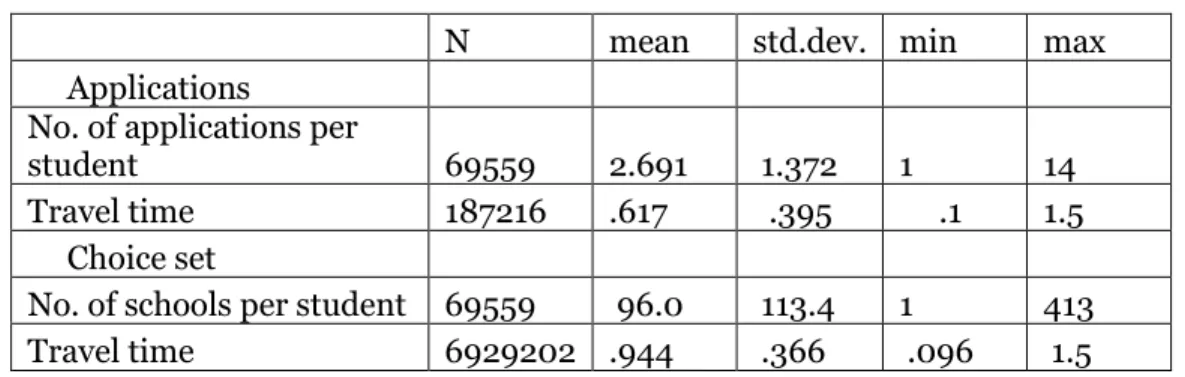
Table 2 compares the set of applications and choice sets. While the average number of applications is 2.7, the average choice set contains 96 schools. The average travel time is also larger within the choice sets.
Table 2 Applications and choice sets
N mean std.dev. min max
Applications
No. of applications per
student 69559 2.691 1.372 1 14
Travel time 187216 .617 .395 .1 1.5
Choice set
No. of schools per student 69559 96.0 113.4 1 413
Travel time 6929202 .944 .366 .096 1.5
RANK-ORDERED LOGIT
Given the nature of the problem, the selection or ranking of schools from a set of schools, we opt for a discrete choice model. A rank-ordered logit model seems most appropriate. The ranking of the schools is modelled as a series of choices from a smaller choice set. The first choice is the most-preferred school in the whole choice set. Removing this school from the set, the second choice is the most-preferred school among all remaining ones, etc.
Imagine a student i ranking schools A, B and C in this way: . This implies his derived utility is highest for school A, followed by B and C: . The probability π we observe this ordering can be written as the product of two probabilities: , with
14
, the set of schools available to the student, and the deterministic part of the student’s utility at school S. This implies the usual, but potentially stringent logit assumptions:
independence of irrelevant alternatives, and extreme value type 1 IID error terms.
To take into account that choices of classmates may be correlated with each other, we estimated robust standard errors clustered at the grade 8 class level.
4. RESULTS
4.1 BASELINE MODEL
We present the results for the most simple linear model in Table 3 below. Students clearly prefer nearby schools. They also prefer schools with higher-scoring peers. In terms of composition, schools with more advantaged student bodies are on average preferred less. This must be interpreted in combination with the school level variable. Preferences for a higher school SES composition would be less negative if the school level variable was not included. Preferences for school quality are small and negative.
Table 3 The most simple linear model
(1)
Simple model Travel time -3.342***
(0.0252) School SES
composition -1.691***
(0.0434) School level 0.546***
(0.0105) School quality -0.0339***
(0.00512) Observations 6929202 Standard errors in parentheses
* p<0.05, ** p<0.01, *** p<0.001
15
The model can be enriched by adding interaction terms (Table4, column 2). The two main candidates are the student’s test score and the student’s SES background (a dummy with cut-off at secondary education). The estimates become more realistic and group dynamics are revealed.
Students from higher educational backgrounds and with higher test scores have a stronger negative preference for distance. They are not willing to travel as far. This could be due to the different geographical location of students. We can check this by including an interaction term capturing travel time to the closest school. This does not significantly change the coefficients for the interaction terms between distance and individual background (coefficients not shown).
Preferences for SES composition, school level and school quality are clearly heterogeneous across groups. High SES and high achieving students prefer a higher SES school composition, higher school level and higher school quality. Preferences for SES composition are relatively more important to high SES students compared to preferences for school level. Preferences for school quality remain small but negative for almost all students (keep in mind that the test score variable is standardized and thus centred around 0). Students clearly have stronger preferences over school level than over school quality.
Table 4 From the simple to the quadratic model
(1) (2) (3) (4)
Simple
model Interaction
terms Quadratic
terms Final
model
Travel time -3.136*** -3.015*** -1.746*** -0.981***
(0.00865) (0.0140) (0.0515) (0.0615)
High SES=1 # Travel time -0.351*** -0.0289 0.0956
(0.0191) (0.0700) (0.0699)
Travel time # Test score -0.231*** -0.141*** -0.0231
(0.0102) (0.0373) (0.0373)
(Travel time)^2 -0.841*** -0.803***
(0.0338) (0.0338)
16
High SES=1 # (Travel time)^2 -0.259*** -0.240***
(0.0470) (0.0468)
(Travel time)^2 # Test score -0.0674** -0.0391
(0.0252) (0.0251) School SES composition -1.748*** -1.991*** 3.210*** 4.249***
(0.0247) (0.0402) (0.135) (0.143) High SES=1 # School SES composition 1.719*** 1.126*** 0.899***
(0.0537) (0.181) (0.179)
School SES composition # Test score 1.003*** 1.547*** 1.423***
(0.0294) (0.0990) (0.0975)
(School SES composition)^2 -6.189*** -6.004***
(0.125) (0.125) High SES=1 # (School SES
composition)^2 0.870*** 0.885***
(0.159) (0.159) (School SES composition)^2 # Test
score -0.415*** -0.394***
(0.0815) (0.0809)
School SES composition # Travel time -1.612***
(0.0656)
School level 0.533*** 0.336*** 0.683*** 0.606***
(0.00584) (0.00979) (0.0128) (0.0177)
High SES=1 # School level 0.0491*** 0.305*** 0.320***
(0.0128) (0.0168) (0.0168)
School level # Test score 0.477*** 0.929*** 0.941***
(0.00667) (0.0103) (0.0102)
(School level)^2 -0.294*** -0.301***
(0.00695) (0.00696)
High SES=1 # (School level)^2 -0.0557*** -0.0547***
(0.00843) (0.00843)
(School level)^2 # Test score -0.0317*** -0.0295***
17
(0.00390) (0.00388)
School level # Travel time 0.0766***
(0.0162)
School quality -0.0215*** -0.0234*** -0.0175** -0.0330***
(0.00289) (0.00450) (0.00534) (0.00824)
High SES=1 # School quality 0.0331*** 0.0213** 0.0243***
(0.00619) (0.00733) (0.00736)
School quality # Test score 0.0344*** 0.0142*** 0.0158***
(0.00345) (0.00403) (0.00403)
(School quality)^2 -0.0810*** -0.0798***
(0.00310) (0.00309)
High SES=1 # (School quality)^2 -0.0199*** -0.0209***
(0.00420) (0.00418)
(School quality)^2 # Test score -0.0399*** -0.0398***
(0.00205) (0.00204)
School quality # Travel time 0.0201*
(0.00828)
Observations 4240322 4206191 4206191 4206191
Standard errors in parentheses
="* p<0.05 *** p<0.001" ** p<0.01
In the next specification (column 3), we add quadratic effects. As the results show, almost all additional terms are highly significant, implying nonlinear utility functions. The quadratic term for travel time is negative: each additional hour (or minute) travelled becomes more of an obstacle. Preferences for higher school SES composition are positive but declining. The optimal school composition is more advantaged for high SES and higher scoring students.
The results for school level and school quality are a bit harder to interpret because they are centred around 0. Preferences for school level are positive but decreasing. Preferences for school quality remain negative. The negative coefficient on the quadratic term implies students dislike the best and the worst schools. At first sight, a negative preference for the best schools may seem implausible. However, if added value is positively associated with expected effort and work load, the negative quality preference may reflect a preference to avoid exerting effort.
18
In the final model (column 4), we add additional interaction terms between travel time and the other main variables. As a result, the travel time coefficient decreases in absolute value. At longer travel times, preferences for a higher SES composition become less outspoken, while preferences for school level and quality become a bit more positive.
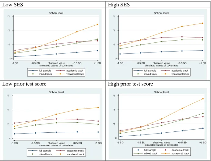
The estimated preferences on our four school choice determinants can be plotted as well. We do this in figures 1 to 4 below. On the horizontal axis, we plot changes in the characteristics of a random school in one’s choice set. On the vertical axis, we plot how this affects the probability that this school is ranked first on the student’s preference list. The graphical representation clearly shows how distance and school level are important characteristics, while school SES composition and especially school quality play a much smaller role. However, we do not see any differences in the preferences for low versus high SES and for low prior test score versus high prior test score (see appendix 8.2).
Figure 1 Preferences for travel time
0.05 .1.15 .2.25
predicted prob. that school is ranked first
-1 SD -0.5 SD observed value +0.5 SD +1 SD
simulated values of covariates
full sample academic track mixed track vocational track
Travel time
19
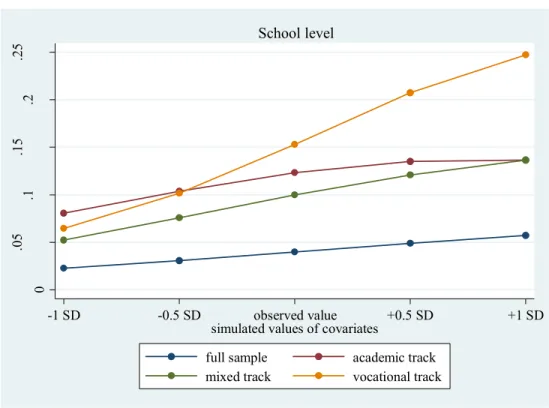
Figure 2 Preferences for school level
0.05 .1.15 .2.25
predicted prob. that school is ranked first
-1 SD -0.5 SD observed value +0.5 SD +1 SD
simulated values of covariates
full sample academic track mixed track vocational track
School level
Figure 3 Preferences for SES composition (to the right means more advantaged)
0
.05 .1.15 .2
predicted prob. that school is ranked first
-1 SD -0.5 SD observed value +0.5 SD +1 SD
simulated values of covariates
full sample academic track mixed track vocational track
School SES composition
20
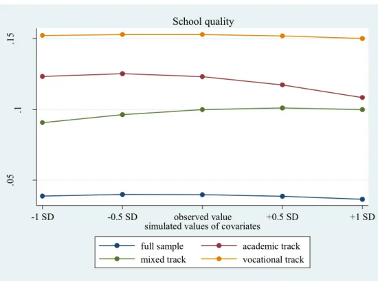
Figure 4 Preferences for school quality
.05 .1.15
predicted prob. that school is ranked first
-1 SD -0.5 SD observed value +0.5 SD +1 SD
simulated values of covariates
full sample academic track mixed track vocational track
School quality
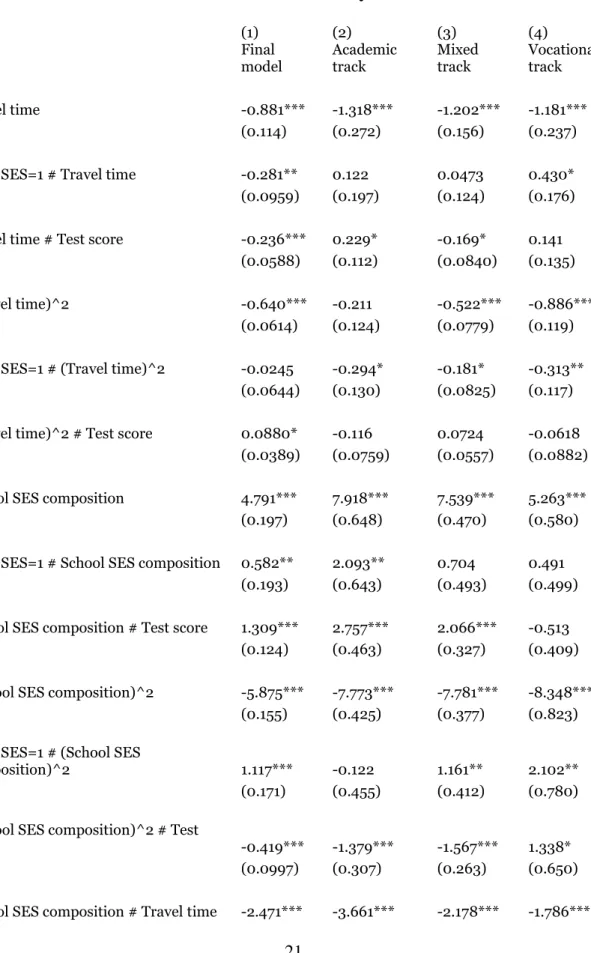
4.2 RESULTS BY TRACK
We run the final model separately by track. Preferences for travel time are more negative in the academic track. This is not because these students live closer to school. When travel time to the closest school is taken into account, the differences between the tracks only increase (estimates not shown). It may be that diversity among vocational programmes in greater, implying that relatively more nearby programmes are rejected by these students.
While school level is more important in the academic track, the baseline coefficient (on the linear term) for school quality takes the expected positive sign only in the mixed track. In the academic and vocational track, quality preferences are negative among the better schools, but students also dislike the worst schools.
21
Table 5 Final model - results by track
(1) (2) (3) (4)
Final
model Academic
track Mixed
track Vocational track
Travel time -0.881*** -1.318*** -1.202*** -1.181***
(0.114) (0.272) (0.156) (0.237)
High SES=1 # Travel time -0.281** 0.122 0.0473 0.430*
(0.0959) (0.197) (0.124) (0.176) Travel time # Test score -0.236*** 0.229* -0.169* 0.141
(0.0588) (0.112) (0.0840) (0.135)
(Travel time)^2 -0.640*** -0.211 -0.522*** -0.886***
(0.0614) (0.124) (0.0779) (0.119) High SES=1 # (Travel time)^2 -0.0245 -0.294* -0.181* -0.313**
(0.0644) (0.130) (0.0825) (0.117) (Travel time)^2 # Test score 0.0880* -0.116 0.0724 -0.0618
(0.0389) (0.0759) (0.0557) (0.0882) School SES composition 4.791*** 7.918*** 7.539*** 5.263***
(0.197) (0.648) (0.470) (0.580) High SES=1 # School SES composition 0.582** 2.093** 0.704 0.491
(0.193) (0.643) (0.493) (0.499) School SES composition # Test score 1.309*** 2.757*** 2.066*** -0.513
(0.124) (0.463) (0.327) (0.409) (School SES composition)^2 -5.875*** -7.773*** -7.781*** -8.348***
(0.155) (0.425) (0.377) (0.823) High SES=1 # (School SES
composition)^2 1.117*** -0.122 1.161** 2.102**
(0.171) (0.455) (0.412) (0.780) (School SES composition)^2 # Test
score -0.419*** -1.379*** -1.567*** 1.338*
(0.0997) (0.307) (0.263) (0.650) School SES composition # Travel time -2.471*** -3.661*** -2.178*** -1.786***
22
(0.113) (0.267) (0.179) (0.262)
School level 0.535*** 1.324*** 0.691*** 0.175
(0.0268) (0.0709) (0.0482) (0.175) High SES=1 # School level 0.352*** 0.240*** 0.0554 0.252
(0.0199) (0.0704) (0.0356) (0.158) School level # Test score 0.970*** 0.915*** 0.899*** 0.635***
(0.0136) (0.0419) (0.0248) (0.133)
(School level)^2 -0.321*** -0.584*** -0.529*** -0.670***
(0.00850) (0.0250) (0.0293) (0.0761) High SES=1 # (School level)^2 -0.0553*** -0.0288 0.0822* 0.0381
(0.00904) (0.0260) (0.0323) (0.0748) (School level)^2 # Test score -0.0306*** -0.00851 0.147*** -0.0455
(0.00489) (0.0141) (0.0202) (0.0629) School level # Travel time 0.182*** 0.345*** 0.269*** -0.0395
(0.0263) (0.0449) (0.0468) (0.0815)
School quality -0.0836*** -0.176*** 0.0487* -0.0713**
(0.0133) (0.0354) (0.0191) (0.0238) High SES=1 # School quality 0.00673 -0.104*** 0.0407*** -0.0241
(0.00840) (0.0226) (0.0122) (0.0138) School quality # Test score -0.0108* -0.143*** 0.0421*** -0.0122
(0.00539) (0.0131) (0.00851) (0.0114) (School quality)^2 -0.0795*** -0.103*** -0.0870*** -0.0322***
(0.00529) (0.0208) (0.00677) (0.00659) High SES=1 # (School quality)^2 -0.0207*** -0.117*** -0.0164* 0.00828
(0.00561) (0.0207) (0.00728) (0.00484) (School quality)^2 # Test score -0.0384*** -0.0251 -0.0326*** -0.0132*
(0.00350) (0.0130) (0.00534) (0.00524) School quality # Travel time 0.0581*** 0.120** 0.0638** 0.0635**
(0.0139) (0.0365) (0.0204) (0.0239)
Observations 6929202 2956351 2574771 1398080
23
Standard errors in parentheses
="* p<0.05 ** p<0.01 *** p<0.001"
4.3 CONSTRUCTING CHOICE SETS
We now consider how students construct their choice sets. Are their preferences for school characteristics the same when students select their highest ranked school and when they select their lowest ranked school? We already indicated that it may not be realistic that students rank all schools they observe. They are likely to only retain the ones they like. In Table 6 below, we show that the preferences inferred from the original choice set are indeed very different from the preferences inferred from the feasible choice set, shown above.
Ideally, we would like to know which schools were considered by the students, and which schools were simply not observed. This information is not available. We thus have to decide on whether to include additional schools into the choice set. Given that most schools will not be ranked, this question implies a choice between two quite different exercises/questions:
1. Within the set of schools that were ranked by the student, why is one school preferred to another?
2. Considering all available schools, why is the set of ranked schools preferred to all other schools? The ordering of the ranked schools still plays a role in this exercise as well, but the larger the number of schools that were not ranked, the lower is the weight on this aspect.
The difference between these questions is shown in Table 6 below. In the first column, we show the results for the final model again. In the second column, we show the estimated coefficients when all ranked schools are considered equally good, but preferred over the non-ranked schools. In the third and last column, we show the results for a model that only considers the original choice sets (i.e. ranked schools). This could be considered as a within-between analysis. The results for our baseline model can be ‘decomposed’ into:
A between component: why are ranked schools preferred over non-ranked schools?
A within component: explaining the rank order among the ranked schools (of course, no equivalent analysis can be done on the set of non-ranked schools)
The coefficients in column 1 and 2 are very similar. The preferences we estimate in the final model (on the feasible choice set) mostly reflect the decision about which schools to rank and which schools not to rank. When we only consider ranked schools, the variation between schools
24
becomes much smaller. This gives rise to less outspoken preferences for school characteristics.
Preferences for travel time and school quality almost vanish, while preferences for school SES composition (same direction but less pronounced) and preferences for school level are more similar to those estimated by the first two models.
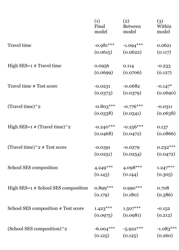
Table 6 "Within and between decomposition"
(1) (2) (3)
Final
model Between
model Within
model
Travel time -0.981*** -1.094*** 0.0621
(0.0615) (0.0622) (0.117)
High SES=1 # Travel time 0.0956 0.114 -0.233
(0.0699) (0.0706) (0.127) Travel time # Test score -0.0231 -0.0682 -0.147*
(0.0373) (0.0379) (0.0690)
(Travel time)^2 -0.803*** -0.776*** -0.0311
(0.0338) (0.0341) (0.0638) High SES=1 # (Travel time)^2 -0.240*** -0.256*** 0.137
(0.0468) (0.0472) (0.0866) (Travel time)^2 # Test score -0.0391 -0.0279 0.232***
(0.0251) (0.0254) (0.0472) School SES composition 4.249*** 4.098*** 1.247***
(0.143) (0.144) (0.305) High SES=1 # School SES composition 0.899*** 0.990*** 0.708
(0.179) (0.180) (0.386) School SES composition # Test score 1.423*** 1.507*** -0.152
(0.0975) (0.0981) (0.212) (School SES composition)^2 -6.004*** -5.922*** -1.083***
(0.125) (0.125) (0.260)
25
High SES=1 # (School SES
composition)^2 0.885*** 0.779*** 0.644
(0.159) (0.159) (0.331) (School SES composition)^2 # Test
score -0.394*** -0.480*** 0.371*
(0.0809) (0.0816) (0.171) School SES composition # Travel time -1.612*** -1.549*** 0.263*
(0.0656) (0.0661) (0.132)
School level 0.606*** 0.588*** 0.923***
(0.0177) (0.0178) (0.0355) High SES=1 # School level 0.320*** 0.329*** -0.0949**
(0.0168) (0.0168) (0.0349) School level # Test score 0.941*** 0.946*** 0.313***
(0.0102) (0.0102) (0.0214)
(School level)^2 -0.301*** -0.305*** -0.165***
(0.00696) (0.00698) (0.0147) High SES=1 # (School level)^2 -0.0547*** -0.0554*** -0.00803
(0.00843) (0.00847) (0.0177) (School level)^2 # Test score -0.0295*** -0.0363*** 0.0446***
(0.00388) (0.00390) (0.00837) School level # Travel time 0.0766*** 0.0922*** -0.238***
(0.0162) (0.0164) (0.0328)
School quality -0.0330*** -0.0298*** -0.0230
(0.00824) (0.00832) (0.0144) High SES=1 # School quality 0.0243*** 0.0240** -0.00648
(0.00736) (0.00739) (0.0131) School quality # Test score 0.0158*** 0.0168*** -0.00418
(0.00403) (0.00405) (0.00742)
(School quality)^2 -0.0798*** -0.0787*** -0.00866
(0.00309) (0.00310) (0.00516) High SES=1 # (School quality)^2 -0.0209*** -0.0215*** -0.00155
26
(0.00418) (0.00419) (0.00697) (School quality)^2 # Test score -0.0398*** -0.0396*** 0.00377
(0.00204) (0.00206) (0.00393) School quality # Travel time 0.0201* 0.0162 0.0317*
(0.00828) (0.00835) (0.0145)
Observations 4206191 4206191 160851
Standard errors in parentheses
="* p<0.05 ** p<0.01 *** p<0.001"
Judging from our estimates when applying the model to the list of ranked schools only (column 3 in the table above, or section 6.1 in the appendix), the probability that a school is included in the student’s ranked list is not random. In particular, we would get very small or even positive coefficients for distance.
We hypothesize that students follow two heuristics when determining their ranking of schools:
1. They do not rank schools that they do not want to attend.
2. Students first rank their most preferred schools and subsequently select backup schools that are nearby.
The first heuristic gives rise to a low variation in school characteristics in the student’s set of ranked schools. Only considering schools that students like will lead to different results, compared to also considering schools they want to avoid. The higher the contrast, the more we can learn about students’ preferences. The second heuristic states that students choose schools from two different sets. They first consider the set of schools they know through their social network and which are attractive options. Then, they select some backup options from the set of nearby schools. Together with the first heuristic, this gives rise to biased estimates on the preference for distance. As the most preferred school may be quite far away, coefficients may even turn out to be positive.
Our final exercise is to find out whether students make different choices when selecting the first and subsequent schools on their list. We study the preferences for school characteristics when students select their favourite school, and when students select the last school on their list.
The results are shown below. They are in line with the second heuristic: students first rank their most preferred schools and subsequently select backup schools that are nearby. Indeed, we find that the preference for nearby schools is stronger when considering the last school on the list.
27
Preferences for school SES composition and school level are less positive. (Preferences for quality are small again and not much different in both cases.) Students will be less likely to select schools with a high SES composition, less likely to select schools with higher performing peers, and more likely to select a nearby school when deciding which school to put at the end of their preference list.
Table 7 Preferences for the first and last school on the student's preference list
(1) (2)
First
school Last school
Travel time -3.077*** -3.417***
(0.0330) (0.0360) High SES=1 # Travel time -0.523*** -0.481***
(0.0356) (0.0379) Travel time # Test score -0.233*** -0.382***
(0.0219) (0.0232) School SES composition -1.580*** -1.970***
(0.0692) (0.0714) High SES=1 # School SES
composition 2.361*** 1.653***
(0.0845) (0.0815) School SES composition # Test
score 0.957*** 1.184***
(0.0485) (0.0487)
School level 0.386*** 0.132***
(0.0160) (0.0171) High SES=1 # School level -0.0355 0.0964***
(0.0191) (0.0193) School level # Test score 0.575*** 0.455***
(0.0109) (0.0112)
28
School quality -0.0269** -0.0271**
(0.00875) (0.00826) High SES=1 # School quality 0.0270* 0.0239*
(0.0106) (0.00947) School quality # Test score 0.0120 0.0270***
(0.00694) (0.00651)
Observations 6929202 6811545
Standard errors in parentheses
="* p<0.05 **
p<0.01 ***
p<0.001"
5. DISCUSSION AND CONCLUSION
In this paper, we investigate how students rank high schools. We infer their preferences for distance, school quality (in terms of value added), school level and school socioeconomic composition. We find that a more advantaged school composition is preferred. Still, these preferences are heterogeneous across social groups, where they are lower for lower social groups.
For high SES and higher scoring students, we find that the optimal school composition is more advantaged. Students and their parents seem to pay much more attention to the level of the school (the average test score of their potential peers) than to school added value. Preferences for the latter are often negative, except among the worst schools and in the mixed track. Higher achieving students even have a stronger negative preference over the schools with the highest added value.
When we look at the school choice process in greater detail, we find evidence for the use of heuristics. To select their favourite schools, students pay more attention to school composition and school level, while in the selection of the remaining schools (back-up options), distance plays a greater role. We also find that the difference between the schools that were selected and the schools that were not selected is very informative if we want to learn about preferences, more than the information in the students submitted preference list.
Our finding that school quality matters is in line with what most other papers have found as well (Lankford and Wyckoff, 1992; Black, 1999; Alderman et al., 2001; Denessen et al., 2005;
Hastings et al., 2008, Dronkers and Avram, 2010; Chumacero et al., 2011; Koning and van der Wiel, 2013; Borghans et al., 2014; Burgess et al., 2014; Cornelisz, 2014). Also the finding that
29
school socio economic composition plays a role in school choice is in line with the previous literature (Lankford and Wyckoff, 1992; Glazerman, 1998; Burgess and Briggs, 2010; Dronkers and Avram, 2010; Burgess et al., 2014; Cornelisz, 2014).
However, the finding that there are differences in characteristics between the favourite schools and other schools on the preference list, as well as the importance of the difference between listed and non-listed schools, seems to be new findings, with which we contribute to the literature.
6. REFERENCES
Alderman, H., P. F. Orazem and E. M. Paterno (2001). School Quality, School Cost, and the Public/Private School Choices of Low-Income Households in Pakistan. The Journal of Human Resources, 36(2), 304-326.
Allen, R. and S. Burgess (2013). Evaluating the provision of school performance information for school choice. Economics of Education Review, 34(1), 175-190.
Biró, Péter (2012), Matching Practices for Secondary Schools – Hungary, MiP Country Profile 6.
http://www.matching-in-practice.eu/secondary-schools-in-hungary/
Black, Sandra E. 1999. “Do Better Schools Matter? Parental Valuation of Elementary Education.”
Quarterly Journal of Economics 114 (2): 577–99.
Borghans, L., Golsteyn, B., and Zölitz, U. (2014). Parental preferences for primary school characteristics. B.E. Journal of Economic Analysis and Policy, Forthcoming.
Burgess, S., Greaves, E., Vignoles, A. and Wilson, D. (2011). ‘Parental choice of primary school in England: what types of school do different types of family really have available to them?’, Policy Studies, vol. 32(5), pp. 531–47.
Burgess, S., Greaves, E., Vignoles, A., & Wilson, D. (2014). “What Parents Want: School Preferences and School Choice.” forthcoming in: The Economic Journal.
Burgess, S. and A. Briggs (2010). School assignment, school choice and social mobility.
Economics of Education Review, 29(1), 649-649.
30
Chetty, R., J. N. Friedman, and J. E. Rockoff (2014) Measuring the Impacts of Teachers I:
Evaluating Bias in Teacher Value-Added Estimates,” American Economic Review,
Cornelisz, I. (2014). School choice, competition and achievement. PhD thesis, Maastricht University.
Chumacero, R. A., D. Gómez, and R.D. Parades (2011). I would walk 500 miles (if it paid):
Vouchers and school choice in Chile. Economics of Education Review, 30(1), 1103-1114.
Denessen, E., Driessena, G. & Sleegers, P. (2005) Segregation by choice? A study of group- specific reasons for school choice. Journal of Education Policy, 20(3): 347-368.
Dronkers, J. and S. Avram (2010). "A cross--‐national analysis of the relations of school choice and effectiveness differences between private--‐dependent and public schools." Educational Research and Evaluation 16(2): 151--‐175.
Elacqua, G. M. Schneider and J. Buckley (2006). School choice in Chile: Is it class or the classroom? Journal of Policy Analysis and Management, 25(3), 577-601.
Glazerman, S. (1998). “School Quality and Social Stratification: The Determinants and Consequences of Parental School Choice.” Unpublished manuscript.
Hastings, J. S., Van Weelden, R. and Weinstein, J. (2007). “Preferences, Information and Parental Choice Behavior in Public School Choice.” NBER Working Paper Series, 12995.
Hastings, J., Kane, T.J. and Staiger, D. (2008). ‘Heterogeneous Preferences and the Efficacy of Public School Choice’, Combines and replaces National Bureau of Economic Research
Working Papers No. 12145 and 11805. Available at:
http://aida.econ.yale.edu/~jh529/papers/HKS_Combined_200806.pdf (last accessed: 24 November 2010).
Hastings, J. and Weinstein, J. (2008). ‘Information, school choice, and academic achievement:
evidence from two experiments’, Quarterly Journal of Economics, vol. 123(4), pp. 1373–414.
Jacob, B., and Lefgren, L. (2007). “What do Parents Value in Education? An Empirical Investigation of Parents’ Revealed Preferences for Teachers.”, Quarterly Journal of Economics, 122 (4): 1603-1637.
Kane, T. J. and D. O. Staiger (2008) Estimating Teacher Impacts On Student Achievement: An Experimental Evaluation, NBER Working Paper No. 14607.
Karsten, Sjoerd, Guuske Ledoux, Jaap Roeleveld, Charles Felix, and Dorothe Elshof. 2003.
“School
31
Choice and Ethnic Segregation.” Educational Policy 17 (4): 452–77.
Koedel, Cory & Kata Mihaly & Jonah E. Rockoff, 2015. "Value-Added Modeling: A Review,"
Working Papers 1501, Department of Economics, University of Missouri
Koning, P. and Van der Wiel, K. (2013). “Ranking the Schools: How Quality Information Affects School Choice in the Netherlands.” Journal of the European Economic Association 11(2) 466- 493.
Lankford, Hamilton, and James Wyckoff. 1992. “Primary and Secondary School Choice among Public and Religious Alternatives.” Economics of Education Review 11 (4): 317–37.
McFadden, D. (1977). ‘Modelling the Choice of Residential Location’, Discussion Paper, Cowles Foundation, Yale University.
Müller, S., S. Tscharaktschiew, and K. Haase (2008). Travel-to-school mode choice modelling and patterns of school choice in urban areas. Journal of Transport Geography, 16(1), 342- 357.
Raudenbush, S. W. and J. D. Willms (1995) The Estimation of School Effects, Journal of Educational and Behavioral Statistics, Winter 1995, Vol. 20, No. 4, pp. 307-335
Ruijs, N., Oosterbeek, H. (2012). “School Choice in Amsterdam. Which Schools do Parents Prefer When School Choice is Free?” Unpublished Manuscript, University of Amsterdam.
32 7. APPENDIX
ALTERNATIVE CHOICE SET SPECIFICATION
The baseline approach of demarcating the choice set in this paper is to include every school within 90 minutes of travel time to the town where the student resides. This is not the only plausible way to proceed. A different approach would be to work with individual-specific choice set radiuses. This is the option we explore in the current section.
For each student, a choice set radius is determined based on the most distant schools that was (explicitly) ranked by the student. A school is now included in the choice set when it satisfies the following conditions:
The school is within reasonable travel time (90 minutes by public transport) from the student’s hometown;
The school was ranked by the student OR
The school was not ranked by the student but
o It is closer to the most distant school that was ranked by the student; and o The type of track was ranked by the student before
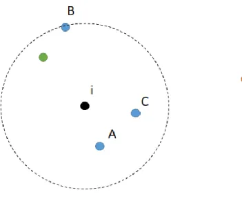
Figure 1 below represents this graphically. Student i ranked three schools: A, B and C. B is the most distant school. The green school is closer to i than school B. If it offers a track that was ranked by i, this track will be added to i's choice set. The orange school will not be considered by i.
33
Figure 8.5 An alternative way of demarcating choice sets
We now present the results of this alternative approach (column 2) and contrast them with our baseline model (column 1). The alternative choice set specification mainly affects the travel time coefficient. Moving from column 2 to column 1 essentially means adding a number of non-preferred, far away schools. The model minimizes the probability that these are chosen by proposing a stronger negative preference for travel time.
Table 8 Comparing results for the baseline model and for an alternative choice set
specification
(1) (2)
Simple
model Individual-specific choice sets
Travel time -3.342*** -0.561***
(0.0252) (0.0277) School SES
composition -1.691*** -1.916***
(0.0434) (0.0440) School level 0.546*** 0.545***