1
Team Research Report, No. MM-2018-1 (Műhelytanulmány, MM-2018-1) Centre for Public Administration Studies Corvinus University of Budapest Hungary
A DDITIVE RAS AND OTHER MATRIX ADJUSTMENT TECHNIQUES FOR MULTISECTORAL MACROMODELS
Krisztián Koppány
1- Tamás Révész
2
1 Széchenyi István University, Győr, Hungary (Széchenyi István Egyetem)
2 Corvinus University of Budapest (Budapesti Corvinus Egyetem)
2
Content
1. Introduction ...4
2. The matrix adjustment problem and its most commonly used solution methods ...6
2.1. The matrix adjustment problem ...6
2.2. The RAS method ...8
2.3. Other matrix adjustment methods ...12
3. Adjustment methods for matrices with negative and zero cells and margins ...14
3.1. Non-sign-preserving methods ...21
3.2. The additive RAS method ...24
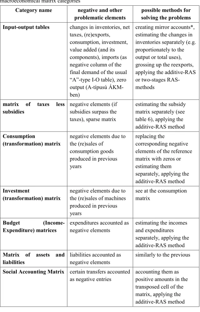
3.3. The model estimating and transforming the 2010 EU I-O tables to GTAP format 32 4. The most important matrices to be adjusted in multisectoral macroeconomic analyses ...37
4.1. Input-output tables “type A” ...38
4.2. Matrices of taxes less subsidies on products ...40
4.3. Transformation matrices of consumption and investment ...42
4.4. Further matrices to be adjusted in the national economy statistics ...44
5. Combined and sequential applications of biproportional matrix adjustment methods ...48
6. Summary ...49
References ...50
3
Additive RAS and other matrix adjustment techniques for multisectoral macromodels
Tamás Révész and Krisztián Koppány Abstract
This paper gives a brief overview of the biproportional matrix adjustment problem.
We focus on the most frequent case with certain and consistent row and column sums, and no special conditions to the cells of the matrix. After the definition and mathematical formulation of the problem, we describe the so-called distance and entropy functions assigning a non-negative real number to the difference of the estimated and reference matrices. These functions are to be minimized subject to given row and columns sums, and in special cases, some non-negativity and sign- preserving conditions. For these models, we present some iterative solution methods, among them the so-called additive RAS algorithm developed and used first by Révész (2001). On one hand, in the case of non-negative reference matrix and positive marginal conditions, one version of additive RAS gives the same solution as the standard RAS, and on the other hand, in the case of negative cells, but sign-preserving margins, another version gives the same solution as the improved normalized squared differences (INSD) model without penalties for sign-switching. We demonstrate that additive RAS is more efficient and more aesthetic than the GRAS and other iterative solution methods used by previous authors. In the case of small differences, additive RAS, especially the flexible version, tends to be sign-preserving, unless it is forced by sign-switches of the margins. Using the example of Lemelin (2009), we demonstrate that additive RAS performs very well even in such an extreme sign-switching case, moreover, it gives the best solution compared to other algorithms. The paper overviews some standard matrix balancing problems in practice, where such methods can be used.
The most important conditions for the successful application are the knowledge about the economic phenomena under investigation and the deep understanding of the related reference matrix. For an example of this, a current research project is presented, where both additive RAS and other more complex adjusting models were used and showed a good performance.
4
Keywords: biproportional matrix adjustment; mathematical programming;
distance function; reference matrix; RAS-method; sign flip; zero margins; least squares; Lagrangian; first order conditions; mean average deviation; input-output table;
Subject classification codes: include these here if the journal requires them
1. Introduction
Estimating the elements of a matrix, when only the margins (row and column sums) are known, is a standard problem in many disciplines. Certain cells can be known (in this case subtracting them from the relating row and column sums, the problem can be converted to the case of unknown cells) or we have only indirect information about them.
Generally, this indirect information is a reference matrix, for which we assume that it has the row and column structure ‘similar’ to the target matrix. The reference matrix can be known counterpart of the target matrix for some previous period or different unit of observation. Similarity, or the opposite of this, can be measured by a ‘distance’ function with the objective to minimize its value.
A typical example is the so-called trip matrix estimation problem. Here, a general xij element of the X matrix denotes the quantity of goods, the number of people transported, or the number of trips between ith and jth places. Performing a full-survey to find out the X for each period can be very expensive and time-consuming. But if we have A, the counterpart of X for some previous period, and the row and column sums of the current X matrix, that is the number of trips originating and terminating in each zone are known for current period, we can try to bend the reference matrix A to these new margins, preserving its structure the best as possible.
Many researchers from several disciplines developed solution strategies to this kind of matrix adjustment problems, in some cases independently, being unaware of other’s achievements. That’s why mathematically equivalent methods are called
5
diversely in distinct disciplines. In transport science these are known as Fratar or Furness (Ortúzar and Willumsen, 2011). In economics the same procedure mainly used for balancing input-output tables is called RAS. This is in the focus of this paper.
The most common methods of the above matrix adjustment problems can be classified into two large groups: the so-called ‘entropy’ models (which contain the logarithm function from the information theory, the classical RAS is also like this) and the models with quadratic objective functions based on the principle of least squares. In the literature a vast discussion emerged about which the method and under what circumstances is more efficient and more reliable. According to experience so far, the best choice depends on the mathematical properties of the reference matrix, target margins, and expectations about the target matrix (non-negativity, zero values, sign switching, sparse matrix etc.), and the economic content of the matrix. Negative and zero values, for example, impede the use of standard methods. Often happens that one of the margins, or some cells of the margins of the adjusted matrix must be zero, while the matrix should continue to contain positive and negative values as well.
The discussion between the authors covered not only the practical application (which method gives better estimates or works more reliably, ensures that the elements of the reference matrix are preserved, for instance), but also the mathematical properties of the techniques (are they biased, do they work in special cases, do they give a unique solution, the same are the solutions of models defined in different ways3 etc.).
This paper briefly overviews these methods and attributes highlighting the mathematical background first, then focusing on the statistical problems and estimation
3 The problem (or the objective function) should be defined in the context of transactions or coefficients, for example, see Mesnard (2011) chapter 4.2.
6
features of matrices in multisectoral modelling practice (various transaction and transformation matrices needed for computable general equilibrium (CGE) models). In this context, special emphasis is given to the ‘additive RAS’ method of Révész (2001) developed for estimating matrices with a negative reference elements and/or non-positive target margins, and the illustration of its efficiency with numerical examples. Based on practical experience and the lessons learned from the literature, we propose ways of further development and future application of estimation methods.
2. The matrix adjustment problem and its most commonly used solution methods
This Section first formalizes the standard matrix adjustment problem, then overviews the two major groups of the proposed solution methods for non-negative matrices, the
‘entropy models’ and the quadratic objective function models, and their relationship.
2.1. The matrix adjustment problem
The matrix adjustment problem most commonly discussed in the literature can be formulated as follows (see for example Lahr and Mesnard (2004), which is the basis for the following review).
Let X* be an m x n unknown matrix, for which row sums are equal to the known u column vector, and column sums are equal to the also known v column vector (that is, X*1 = u, 1TX* = v, where 1 is the summation vector and T denotes transpose).
If we also have an m x n reference matrix A (also known as prior), which is similar to X* in its structure, then it can be estimated with the matrix X, also of the size m x n, which has row sums equal to the column vector u and column sums equal to v (i.e., X1 = u, 1TX = v), such that X is the most similar to the reference matrix A in some sense.
7
In the paragraph above, the use of the term ‘structure’ is justified by the following considerations. Of course, depending on the definition of the ‘similarity’ (or the
‘deviation’ or ‘distance’) of the two matrices (A and X), the solution to the problem (X) may be different. Even if we lock the formula for comparing the two matrices, the solution will naturally continue to depend on the reference matrix A. If, however, it depends not only on the structure of A (the internal proportions of its elements), but also on its ‘level’
(that is, multiplying A by a γ scalar yields different solution), then it is advisable to first modify A (proportionally adjust by multiplying by the γ scalar) that grand total (1TA1) are equal to the grand total of (1TX*1), i.e. 1TA1 = 1Tv = u1. This makes it only possible that if with this equal scaling, conditions A1 = u and 1TA = v are also fulfilled, the modified reference matrix A is the solution X itself. ‘Levelling’ of the reference matrix A reduces or (if it meets the conditions) eliminates the need for further correction.
Of course, with a given formula of the ‘similarity’ of two matrices, it is possible that the problem has several solutions for which this formula gives the same value.
However, if A is irreducible, the set of possible solutions is compact, and the objective function can be continuously differentiated over that set, there is only one solution, which is true for the methods involved here (Mesnard, 2011). This problem is not discussed in general in this paper, however, we will return to the point when discussing the concrete formulae of ‘similarity’.
In any case, the matrix adjustment task can be defined as a mathematical programming problem, where the goal is to find the optimal value of the target function (the maximum of the similarity formula or the minimum of a monotonous increasing function of the deviation), subject to the constraints X1 = u and 1TX = v (and possibly some nonnegativity or sign-preservation conditions). If the constraints are linear, the optimum can be determined by the method of the Lagrangian multipliers. In the
8
Lagrangian function, these multipliers penalize for deviations from constraints and express how much a unit increase in constraints changes the optimum value. Some authors initially start from the Lagrangian function, but modify it, for example, by introducing deviations from constraints not only by multiplying the corresponding Lagrange multiplier, but by logarithm of the resulting multiplications, see, for example, Günlük-Şenesen and Bates (1988). This has benefits in the entropy models with logarithmic objective functions, if so the relations between the element of the reference matrix and the λi and τj Lagrangian multipliers for the deviations from the prescribed row and column sums can be expressed in a simple multiplication form of xi,j = ai,j ∙ λi ∙ τj in the solution (although not optimal for the original program) generated by the first-order conditions.
One can raise that instead of looking at how much the initial structure is preserved;
the method should rather be looked at as to how much it changes elements of the prior in line with the expected changes in the margins. For example, if both the row and the column sums increased, then it is a legitimate expectation that the element at the interSection of them also increases (of course, only to the justified extent). This issue will be concerned in the next chapters, but we cannot undertake general discussion. In any case, it is worth thinking about compiling a criteria system that examines such and similar aspects.
2.2. The RAS method
The most obvious solution algorithm for the matrix adjusting problem is the RAS method, which was first documented in the 1930s, used in input-output modelling in the 1940s and was disseminated in economic literature by Sir Richard Stone (Stone 1961, Stone and Brown 1962).
9
The first step of the RAS iteration process is to multiply the rows of matrix A by the corresponding ratio of the prescribed and the actual row sums ui/bi (where b denotes the column vector of actual row sums, and bi is the ith element of b for row i), hence adjusting the matrix horizontally to u, the vector of target row sums. Then the columns of the resulting matrix should be multiplied by the corresponding ratio of the prescribed and the actual column sums vj/sj (where s denotes the column vector of actual column sums, and sj is the jth element of s for column j), hence adjusting the matrix vertically to v, the vector target column sums.4 The second iteration starts with A1, the resulting matrix of the first iteration, and so on and on. Thus, in the ith step one can obtain matrix Ai performing the row and column direction adjustment referred to above on the matrix Ai-
1, the result of the (i-1)th iteration. This process is usually convergent.5
The limit of the matrix sequence Ai yields X, which is the solution of the following mathematical programming problem (Bacharach 1970)6:
X1 = u, 1TX = v,
m
i 1
n
j 1
xi,j ln(xi,j/ai,j) –> min. (1)
The solution of (1) using the method of Lagrangian multipliers one can obtain
X = rr rrˆ A s ˆ, (2)
4 The order of row and column adjustments can be interchanged, the final solution is not affected.
5 The necessary and sufficient conditions for convergence were demonstrated by MacGill (1977), see also Lemelin et al. (2013).
6 According to Schneider and Zenios (1990) this corresponce was proved by Bregman (1967) before Bacharach (1970).
10
where ˆ denotes the diagonal matrix of a vector, and r and s are the vectors generated from the shadow prices of the constraints X1 = u and 1TX = v, respectively (Bacharach 1970).
Since the target function is convex and can be continuously differentiated on a compact set, if matrix A is indecomposable (Zalai 2012), then the solution X = rr ˆA s ˆ is unique, except for any arbitrary δ and 1/δ scalar multipliers for r and s vectors (Bacharach 1970, Mesnard 2011). This means that if a r and s vector pair is a solution, then the r∙δ and s/δ vector pairs are also.
Thus, the RAS method is a biproportional technique, which adjusts the original matrix on one hand, by rows, and on the other hand, by columns with uniform multipliers (within the given row or column).
The objective function (1) of the RAS method is also known as an information loss formula of the information theory.7 Lemelin et al. (2013) clearly shows that RAS is equivalent to the following task
m
i 1
pi,j = p.,j,
n
j 1
pi,j = pi,. ,
m
i 1
n
j 1
pi,j ln(pi,j/pai,j) –> min, (3)
where pai,j = ai,j /1TA1, pi,j = xi,j/w , p.,j = h,j /w , pi,.= ui /w, and w = u1 (i.e., the prescribed grand total of the elements of matrix X). Thus, pi,j‘s are considered to be elements of a two-dimensional joint probability distribution, and the target function is the ‘additional’
information contained by the probability distribution pi,j relative to the probability distribution pai,j. The tasks and their solution techniques that can be formulated the way
7 The mathematical formulation of information theory was developed by Shannon (1948) and was introduced to economics by Theil (1967).
11
above are called cross-entropy problems and methods.8 Thus, the RAS method is a special case of cross-entropy methods.
By generalizing the deduction of Lemelin et al. (2013) it can be easily shown that the RAS method leads to the same result even if the reference matrix A is multiplied by any positive number. Multiplying by a γ scalar we obtain the objective function
m
i 1
n
j 1
xi,j ln(xi,j/(γai,j)) =
m
i 1
n
j 1
xi,j{ln(xi,j/ai,j)– ln γ} =
m
i 1
n
j 1
xi,j ln(xi,j/ai,j)– w ln γ,
which differs from the original objective in only one constant, thus, it has the same minimum point. Thus, from the mathematical point of view it does not matter whether the matrix A is multiplied by the γ = w /1TA1 scalar to ensure that the grand sum of it is equal to the sum of the target margins. Of course, it is a very different question whether it is worthy to modify matrix A to A* to satisfy the marginal constraints A*1 = u, 1TA* = v, that is to be a possible solution to the problem (1) at sight. Another question is, which of the lot of possible modifications should be chosen (the degree of freedom is considerable, since we have only n+m-1 independent conditions for the m x n elements of the reference matrix). Thus, we can reach the problem of the two-stage matrix estimation, in which case in the first stage matrix A is adjusted to the optimal A*, then using this as the reference matrix we generate the final estimate of the matrix X with a secondary adjustment model. It can be argued that the models used in the two stages should be "harmonized" (theoretically coherent) or deviated (using a completely identical model, there is clearly no point in breaking the process into two stages, since every
8 The concept of cross-entropy was introduced and discussed first by Kullback and Leibler (1951).
12
optimization process starts computing by finding a possible solution).
2.3. Other matrix adjustment methods
Even in the case of nonnegative matrices, there are a variety of objective functions, different from the loss of information described above, that can be used and justified for the matrix adjustment problem. A very similar function is
m
i 1
n
j 1
ai,j ln(ai,j/xi,j), which just revers the cast between the elements of the reference and the target matrix. For the comparative analysis of the results, see for example McNeil and Hendrickson (1985). The advantage of this objective is that each variable xi,j only appears once in the formula, so it is easier to calculate and its mathematical properties (monotony, non-negativeness, etc.) are easier to understand.
The basic versions of the so-called gravity models, mainly used for estimating the transport matrix,9 see for example, Niedercorn and Bechdolt (1969) and Black (1972), can be considered equivalent to the RAS method, too (Mesnard 2011).
We do not mention here any possible, differently weighted objective functions that contain logarithm functions, but instead turn to the ‘least squares’ target functions.
According to Lahr and Mesnard (2004), Pearson's χ2 or the normalized quadratic deviation (the method of normalized least squares) was first used by Deming and Stephan (1940) and Friedlander (1961) to solve the matrix adjustment problem, and it was also suggested by Lecomber (1975) to update symmetric input-output tables (SIOTs). The
9 The transportation problem is to deliver the quantity xi,j of the product x from the ith the starting point having a stock of ui to the jth destination point demanding the quantity of vj so that the transport cost is minimal.
13
objective function to minimize can be formalized by the two following and equivalent ways:
m
i 1
n
j 1
(xi,j – ai,j)2/ai,j =
m
i 1
n
j 1
(xi,j /ai,j –1)2∙ai,j. (4)
The second formula shows that this objective function represents the squared sum of the relative (%) difference of estimated and original matrix elements weighted with the original matrix elements. This means a compromise between Almon’s (1968) simple sum of squared deviations10
m
i 1
n
j 1
(xi,j – ai,j)2 (5)
and the unweighted relative squared sum
m
i 1
n
j 1
(xi,j /ai,j –1)2 =
m
i 1
n
j 1
( xi,j – ai,j)2/ai,j2. (6)
It is easy to see that the simple square sum is likely to allow larger deviations at the small elements, while the unweighted relative square deviation is vice versa, the quantities to be distributed (the amount to be added or subtracted for the required row and column sums) are to be divided into larger elements, where the adjustment means a smaller percentage value.
10 Although Almon used this formula for the coefficients of the input-output table, i.e. instead of the marginal constraints X1 = u, 1TX = v, he minimizes the objective function subject to X g
= u, 1TX rr rgˆ = v, where g is the vector of known gross sectoral outputs.
14
As a generalization of the squared deviations and summarizing with weights 1, 1/ai,j and 1/ ai,j2 (i.e. the objective functions (4)-(6)) Harthoorn and van Dalen (1987) introduce
m
i 1
n
j 1
( xi,j – ai,j)2/gi,j
where weights 1/gi,j represents the ‘relative confidence’ of the elements ai,j, regarded as
‘first approximations’ (Timurshoev et al. 2011).
It is also easy to see that the objective functions based on square variances, in contrast to the entropy (log) functions, allow the estimated xi,j to be different sign from the original ai,j. Likewise, it is obvious that the original zero elements may also become non-zero. These issues will be discussed in the following Section.
3. Adjustment methods for matrices with negative and zero cells and margins In this Section firstly, we present some modifications of methods for biproportional matrix adjustment discussed in the Section 2. These modifications are necessary to apply the methods in cases when there are negative entries in the reference matrix and/or there are negative or zero element in the prescribed row and column vectors.
The database of a multisectoral economic model often includes a cross-table (or contingency table) of such deaggregated categories. If these are to be estimated, in many cases, negative or zero values hinder the use of standard methods. For example, if the target value of a complete row or column margin (or some elements of it) is zero, the RAS estimation would set the entire row or column to zero in the first iteration, even if there are in fact both positive and negative values that are obviously and significantly different from zero, and their signs should be preserved. It is no better luck if one of the row or column sums of the reference matrix is zero (of course, then either all elements of
15
the row or column must be zero or there must be positive and negative elements, as well), but the corresponding required margin value is zero. To highlight the weight of the problem, it is worth noting that the RAS algorithm that is otherwise not recommended in this case, would attempt to divide by zero when proportionally adjusting the given row or column.
As can be seen from their formulas in Section 2, the matrix correction methods discussed so far do not work or fail if some element of the reference matrix or one of the prescribed row or column sums is negative. Except for the banal ad hoc treatments of these problems, such as the replacement of the small negative ai,j elements to zero (Omar 1967)11, or leaving them unchanged, Günlük-Şenesen and Bates (1988) and re- discovering their results, Junius and Oosterhaven (2003) first deals thoroughly with the treatment of the negative elements. The objective function of their ‘generalized RAS’
(GRAS) method
m
i 1
n
j 1
|ai,j|∙xi,j /ai,j∙ln(xi,j/ai,j)
is distorted (Huang et al. 2008) and cannot be applied if not all columns and rows have a positive element (Temurshoev 2013), or as we will see, even in normal cases it does not always give the best results among the estimation methods available. Later on, Oosterhaven (2005) himself also points out that negative and positive differences can be eliminated in the originally proposed objective function (creating the illusion of perfect fit) and instead of it, he proposes the
m
i 1
n
j 1
|ai,j∙xi,j /ai,j∙ln(xi,j/ai,j)| absolute information
11 Quoted by Lahr and Mesnard (2004).
16
loss (AIL) function. Later again, the distortion of the GRAS objective function is corrected by Lenzen at al. (2007).12 Huang et al. (2008) further changes the objective function to
m
i 1
n
j 1
|ai,j|∙(zi, j ∙ln(zi, j /e) +1), and name this ‘improved GRAS’ (IGRAS).
They add a constant to the function, with which in the case of zi, j = 1 it will be zero, but this does not affect the location of the optimum.
In any case, it can be seen from the logarithm in the objective function that if the model has any solution, for every i, j pairs xi,j/ai,j = zi,j ≥ 0 holds. Thus, the solution of the GRAS model guarantees that matrix elements preserve their sign (that is, the signs of the estimated matrix are the same as the reference matrix).
In addition to the entropy models based on some quantity of information, in the models containing quadratic objective functions can be formulated to preserve the signs of the reference matrix. Jackson and Murray (2004), for example, minimizes the following objective function (see their Model 10)
m
i 1
n
j 1
|ai,j|∙xi,j /ai,j∙ln(xi,j/ai,j),
where zi,j = xi,j/ai,j, subject to the usual marginal conditions and the zi,j ≥ 0 nonnegativity constraint. This so-called ‘sign-preserving squared differences’ model can be solved by the commercial mathematical programming softwares (for example the GAMS), but the inequality conditions do not allow to derive the optimal solutions using the method of
12 The function zln z has its minimum at the value z = 1/e, where e is the Euler-number (the base of the natural logarithm) and z denotes the ratio xi,j/ai,j. The minimum point should be z = 1.
Function zln(z/e) proposed by Lenzen at al. (2007) indeed has its minimum at z = 1.
17 Lagrangain multipliers.
Maybe that is why Huang et al. (2008) prevents the switch of the sign of the matrix elements in an alternative way. They use an additional +M/2 ∙
m
i 1
n
j 1
|ai,j|∙ (min(0, zi,j )) 2 component in the Lagrangian function, where M is a sufficiently large positive number.
The numerical example of Junius and Oosterhaven (2003), constructed for adjusting a matrix with partly negative entries and marginal values, is used by several authors for the empirical analysis of the ‘goodness of fit’ of the competing methods, based on a variety of ‘assessment’ criteria. From these methods, Jackson and Murray (2004) have found the above-mentioned ‘sign-preserving squared differences’ model as the best.
Similarly, Huang et al. (2008) also concluded that the so-called ‘improved normalized square deviation’ (INSD) objective function
m
i 1
n
j 1
(xi,j /ai,j –1)2∙|ai,j| +M/2 ∙
m
i 1
n
j 1
|ai,j|∙(min(0, zi,j ))2 (7)
shows the best performance (on average) using the example of Junius and Oosterhaven (2003). This, in addition to good estimation results, basically supports the justification for the similar (quadratic-type) target function chosen by the EU-GTAP project (Rueda–
Revesz et al. (2016)).
As pointed out by Huang et al. (2008), and as Temurshoev et al. (2011)) has been deduced precisely, the INSD objective function is the first term of Taylor-series of the IGRAS objective function at zi, j =1, that is
|ai,j|∙(zi, j ∙ln(zi, j /e) +1) ≈ |ai,j|∙(0 + zi, j ∙ (zi, j –2) +1) ≈ |ai,j| ∙ (zi, j –1)2.
18
Therefore, and since in GRAS estimates zi, j ≥ 0, Huang et al. (2008) claim that the INSD method is more prone to preserve the sign of elements than other non- biproportional methods.
In addition to the above and the empirical testing, Huang et al. (2008) gives the Lagrange functions associated with the constrained optimization problem corresponding to each method and derives the formulas of optimum solutions.13 In the case of INSD, these are the following:
zi,j =
1 , = 0
1 + ( , )ž( + ) ℎ = 0
0 1 + , ž + < 0 → ∞
, (8)
λi ={(ui – Ʃj ai,j) + Ʃj (M ∙ ai,j ∙ min(0, zi,j ) – τj ∙|ai,j|)} / Ʃj|ai,j|, and (8a) τj ={(vj – Ʃi ai,j) + Ʃi (M ∙ ai,j ∙ min(0, zi,j ) – λi ∙|ai,j|)} / Ʃi|ai,j|, (8b) where zi,j = xi,j /ai,j, and λi and τj are the Lagrangian multipliers belonging to the row- and column sum deviations.
If zi,j ≥ 0, that is ai,j doesn’t change its sign, the formulae for λi és τj simplify to the following forms:
λi ={(ui – Ʃj ai,j) – Ʃj (τj ∙|ai,j|)} / Ʃj|ai,j|, and (9)
13 The errors in the first order conditions were corrected later by Temurshoev et al. (2011), but they also do not justify the division of the target function by 2 in the Lagrange function, which is equivalent to double-weighting the penalty function for deviations from margins.
19
τj ={(vj – Ʃi ai,j) – Ʃi (λi ∙|ai,j|)} / Ʃi|ai,j|. (10) It appears from the middle part of the formula (8) for the definition of zi,j, that the Lagrange multipliers should be added in the case of positive, and should be subtracted in the case of negative ai,j elements.
Multiplying the middle part of (8) by ai,j yields
xi,j = zi,j ∙ ai,j = ai,j + ai,j ∙sgn(ai,j)∙( λi + τj). (11) Introducing di,j = xi,j – ai,j, subtracting ai,j from each side of (10), and considering that ai,j
∙sgn(ai,j) = |ai,j|, we obtain
di,j = xi,j – ai,j = |ai,j|∙(λi + τj) (12) expressing the relation between the Lagrangian multipliers and the (optimal) changes of the elements of the matrix.
From the equations (9) and (10), these multipliers depend on each other, and the row and column direction absolute value share of the element, as well.
It is also worth noting that similarly to the RAS method (where the Lagrangian multipliers of the rows and columns can change inversely in groups, and uniformly, but in any proportion within a group), it is apparent from formula (12) that it leads to the same estimate when choosing any φ value for λi replacing λi + φ and replacing τj with τj – φ, they still satisfy (8), (9) and (10). So in this sense, if there is a solution, there are infinite
ones, but while in case of a ‘multiplicative’ RAS, the degree of freedom of the Lagrangian multipliers occurs in a proportionality factor, while for the INSD in an additive component.
Since in the general (sign-preserving) case discussed by Huang et al. (2008) equations (8)-(10) are simultaneous (λi and τj depend on each other and zi,j, and vice
20
versa), they suggest an iterative solution algorithm with zi,j(0) =1, λi(0) = 0, τj(0) = 0 initial values. In the not sign-preserving case discussed later in Section 3.2., however, λi and τj
depend on each other only. In the first iteration suggested by Huang et al. (2008), according to equations (9) and (10) the Lagrangian multipliers are
λi(1) = gi / Ʃj |ai,j| (13)
τj(1) = hj / Ʃi |ai,j| (14)
where gi = ui – Ʃj ai,j and hj = vj – Ʃi ai,j denote the differences of the prescribed row and column sums from those of the matrix A.
Now take S = |A|, where |A| denotes the matrix containing the absolute values of the elements of A, w = 1TS, q = S1, and R = q ˆ-1S and C = S w ˆ-1 , ,, where R and C are matrices containing the row- and column-wise absolute value distribution of S.
Substituting (13) and (14) into (12) we obtain that in the first iteration the elements of the matrix change by
di,j(1)= |ai,j|∙(λi(1) + τj(1)) = gi ∙|ai,j| / Ʃj |ai,j| + hj∙|ai,j|/ Ʃi |ai,j| = gi ∙ri,j + hj∙ci,j. (15) This means that the iteration adjusts the rows and columns of the matrix by the row- and column-wise absolute value share of the elements.
Note, that the first step of the iteration would add the discrepancy (do the adjustment to the target margins) ‘twice’, in the
m
i 1
n
j 1
di,j(1) =
m
i 1
gi +
n
j 1
hj formula of the overall total of the resulting matrix both the
m
i 1
gi , and the
n
j 1
hj components alone would eliminate the overall discrepancy. We will come back to this issue in section 3.2.
21
Using the recently introduced notations multiplying equations (9) and (10) (which determine the optimal values of λi and τj) by qi = Ʃj|ai,j| and wj = Ʃi|ai,j| respectively we get their
λi ∙ qi = gi – Ʃj (τj ∙si,j) (16)
τj ∙ wj = hj – Ʃi (λi ∙si,j) (17)
simpler versions. With matrixalgebraic notations (16) and (17) can be combined into the ˆ
ˆ = (18)
system of inhomogenous linear equations, where λ, τ, g and h are the column vectors containing the λi , τj, gi and hj elements respectively.
Since 1Tg = 1Th , qˆ 1 = q = S1 and w ˆ 1 = w = ST1 , therefore the following holds:
ˆ
ˆ − = (19)
Since (19) can be interpreted as a solution of a homogenous system of linear equations, its ˆ
ˆ (symmetric) coefficient matrix (denoted subsequently by S*) is singular (i.e.
its rows/columns are linearly interdependent). Therefore the (18) system of linear equations cannot be solved by multiplying it from the left by the (non-existent) inverse of the S* matrix. Instead, one must express one variable by the rest and must be dropped along with the corresponding equation. Finally, the reduced set of linear equations (which contains (m+n-1) equations and the same number of variables) can be solved by multiplying it from the left by the (non-existent) inverse of the reduced coefficient matrix.
3.1. Non-sign-preserving methods
Estimates of the matrices with negative entries can easily be a sign-switching. Previously, the authors tried to avoid this with using sign-preserving algorithms. It was needed
22
especially in entropy models because the logarithmic objective function is not defined in case of negative zi,j. However, there may also be cases where the required marginal values are such that the signs of the elements ai,j and xi,j, must be different.
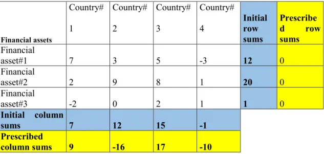
Lemelin (2009) also presents such a case when attempting to extend and test the GRAS, ant the Kullback and Leibler (1951) cross-entropy methods for zero-margin matrices. In his study the numerical example of Junius and Oosterhaven is first interpreted as a net world trade matrix, where the element ai,j of the inconsistent initial matrix A shows the net exports of the ith country from the ith product. The row and column sums of the estimated X matrix must be zero. Then, the example changes to the matrix of net investment positions, where ai,j represents the net claim of the jth country from ith asset.
In the latter case, the row sums of X must also be zero, but in the column sums there may be negative values, as well. That is why Lemelin determined the prescribes a negative target sum for column 2 with originally positive elements to force the sign-switch of some elements, and to test Kullback and Leibler’s cross-entropy, and Junius and Oosterhaven's GRAS methods, somewhat modified to these cases. Table 1 shows the initial matrix and required row and column sums.
Table 1. Initial matrix of net international investment positions and prescribed margins
Financial assets
Country#
1
Country#
2
Country#
3
Country#
4
Initial row sums
Prescribe
d row
sums Financial
asset#1 7 3 5 -3 12 0
Financial
asset#2 2 9 8 1 20 0
Financial
asset#3 -2 0 2 1 1 0
Initial column
sums 7 12 15 -1
Prescribed
column sums 9 -16 17 -10
23
Table 2 shows the matrix X estimated with cross-entropy method.
Table 2. Adjusted matrix of net international investment positions using cross-entropy model
Financial assets
Country#1 Country#2 Country#3 Country#4 Estimated row sums
Prescribed row sums Financial
asset#1 27495.08 -36579.17 24854.35 -15770.26 0 0 Financial
asset#2 -11049.53 36563.17 -34936.82 9423.19 0 0
Financial
asset#3 -16436.55 0 10099.48 6337.07 0 0
Estimated
column sums 9 -16 17 -10
Prescribed
column sums 9 -16 17 -10
Lemelin explains the apparently unrealistic results of the cross-entropy method by that the method seeks to preserve the proportions of the elements of the matrix. Thus, even if small column sums are to be corrected at a higher rate, the relating column entries change at the same large scale (like RAS).
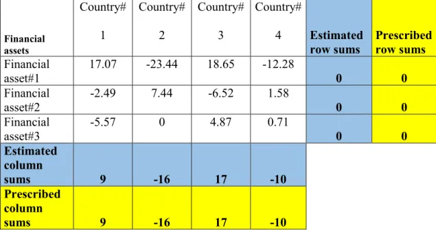
Using the GRAS method, Lemelin obtained the following results (see Table 3 here, and Table 8 in Lemelin 2009).
Table 3. Adjusted matrix of net international investment positions using GRAS model
Financial assets
Country#
1
Country#
2
Country#
3
Country#
4 Estimated row sums
Prescribed row sums Financial
asset#1
17.07 -23.44 18.65 -12.28
0 0
Financial asset#2
-2.49 7.44 -6.52 1.58
0 0
Financial asset#3
-5.57 0 4.87 0.71
0 0
Estimated column
sums 9 -16 17 -10
Prescribed column
sums 9 -16 17 -10
24
Comparing the results obtained with the two methods, Lemelin states that the modified GRAS method proved to be better than the cross-entropy method. Unfortunately, he did not investigate the solutions available with quadratic-type targeting functions, although they obviously allow for sign-switching. We will address this issue in next section.
After discussing reasons for changes in inventories (which products and how often change in the related column of the input-output tables), Lenzen (2014) reverses the general negative judgement of the sign-switching and looks as an advantage that, if necessary, an adjustment process can change the sign of the elements of the reference matrix.
3.2. The additive RAS method
In the turbulent early years of economic transition of the Hungarian economy (the early 90s) while trying to update the Hungarian input-output tables, its auxiliary matrices and other macroeconomic matrix categories I developed my “additive-RAS” algorithm (Révész, 2001) and used it instead of the RAS in the case of zero (or close to zero) known (target) margins or negative reference matrix elements of unpleasant magnitude and appearing in unlucky locations (in which cases the RAS is unusable or at least unreliable).
In the first step this additive-RAS algorithm for each row distributes the difference of the target row total and the corresponding row-total of the reference matrix proportionately to their row-wise absolute value share (as matrix R was defined above) according to the
xi,j(1)(r) = ai,j + gi(1) ∙ri,j (20)
formula, where gi(1) = gi . Then a similar adjustment has to be done column-wise according to the
xi,j(1) = xi,j(1)(r) + hj(1)∙ci,j (21)
formula, where hj(1) = vj – Ʃi xi,j(1)(r).
25
In general, the n-th iteration (i.e. which contains the n-th row-wise and n-th column-wise adjustment) can be described by the
xi,j(n)(r) = xi,j(n-1) + gi(n) ∙ri,j (22)
(where gi(n) = ui – Ʃj xi,j(n-1)) and
xi,j(n) = xi,j(n)(r) + hj(n)∙ci,j (23)
formulas, where hj(n) = vj – Ʃi xi,j(n)(r). Based on this the total change in the individual elements, caused by the first n iteration ( di,j(n) = xi,j(n) – ai,j ) can be described as
di,j(n) = ∑ ( ( )∙ , + ℎ( )∙ , ) = ri,j∙∑ ( ) + ci,j ∙ ∑ ℎ( ). (24) If the process converges then obviously its di,j(∑) limit value can be computed as
di,j(∑) = ri,j∙ gi(∑) + ci,j ∙ hj(∑) (25) where gi(∑) = lim
→
(∑) and hj(∑) = lim
→ ℎ(∑).
Since the di,j(∑) elements of the ‘final’ matrix should satisfy the row-total and column-total requirements (otherwise the adjustment process would continue by distributing the remaining discrepancy), summing the equations of (25) by j we get the following:
gi = Ʃj di,j(∑) = Ʃj (ri,j∙ gi(∑)+ ci,j ∙ hj(∑)) = gi(∑) ∙Ʃj (ri,j + ci,j ∙ hj(∑)) = gi(∑) +Ʃj (ci,j ∙ hj(∑)) (26) Similarly summing the equations of (25) by j we get the
hj = Ʃi di,j(∑) = Ʃi (ri,j∙ gi(∑)+ ci,j ∙ hj(∑)) = Ʃj (ri,j∙ gi(∑)) + hj(∑)∙Ʃi ci,j = Ʃj (ri,j∙ gi(∑)) + hj(∑)
(27)
conditions for the so far unknown gi(∑) and hj(∑) values. Equations (26) and (27) can be described in matrixalgebraic notations as
g = g(∑) + C h(∑) = q ˆ q ˆ-1g(∑) + S w ˆ-1 h(∑) (28) h = RT g(∑) + h(∑) = ST q ˆ-1g(∑) + w ˆ w ˆ-1h(∑) (29)
26
respectively, where g(∑) and h(∑) mean the column vectors containing the elements of gi(∑) and hj(∑) respectively. Equations (28) and (29) can be combined in the
ˆ ˆ
ˆ (∑)
ˆ (∑) = (30)
system of inhomogenous linear equations.
Comparing this with (18) we can see that both the coefficient matrices and the right-hand-side constant vectors are the same as their counterpart in (18) and (30).
Therefore the solutions of the (18) and (30) set of linear equations are the same too. This means that if λ, τ are the solution of (18), then those g(∑) and h(∑) vectors which satisfy the q ˆ-1g(∑) = λ and w ˆ-1 h(∑) = τ equations, hence which can be computed as
g(∑) = q ˆ λ (31)
h(∑) = w ˆ λ (32)
are the solutions of the (30) set of linear equations. By substituting (31) and (32) into (25) we get the
di,j(∑) = ri,j∙ qi ∙ λi + ci,j ∙ wj ∙ τj = si,j∙ λi + si,j ∙ τj = |ai,j|∙( λi + τj) (33) formula for the resulting total changes (in the individual matrix elements) of the additive- RAS algorithm. This is just the same as (12), i.e. what for this case Huang et al (2008) derived as the optimal solution of the INSD-model.
Therefore, we proved that the result of the additive-RAS algorithm is identical to that of the INSD-model if the sign of the matrix elements do not change. Fortunately, sign flips occur only if the ratio of the target- and actual margins is extremely high. For example, (since the shares in the absolute values are smaller than the value shares) unless this ratio falls below -100 per cent, the iteration certainly does not cause sign flips. This is true in the case of even more extreme margin adjustment ratios. In any case, extreme
27
margin adjustment ratios raise concern about the applicability of the reference matrix, i.e.
about whether the structure of the searched (target) matrix may preserve the similarity to the structure of the reference matrix.
The above ‘shares in the absolute values are smaller than the value shares’
statement requires certain qualifications. This is true only if they are computed from the same matrix. In the above presented algorithm the absolute value shares are computed from the ai,j elements of the reference matrix, while the ‘actual’ value shares (i.e. in the n-th iteration) are computed from the already adjusted xi,j(n)(r) and xi,j(n) matrices.
Therefore, if for some reasons the structure of the xi,j(n)(r) and xi,j(n) matrices differ considerably from the structure of the reference matrix then the additive RAS algorithm may cause sign flips. Although the algorithm still may converge and may produce apparently reasonable results, it can not be guaranteed that these results are the best estimates according to some usual optimum criteria (distance measure).
Hence if the additive-RAS algorithm produces sign flips and consequently its mathematical characteristics become opaque (unclear) then it is worth modifying the algorithm appropriately. Concretely – similarly to what practically the multiplicative RAS algorithm does with the value shares, - we may compute the absolute value shares from the n-th iteration’s (‘current’) xi,j(n)(r) and xi,j(n) matrices (more precisely we denote these by x˜ i,j(n)(r) and x˜ i,j(n) respectively, since these differ from their counterparts in the original additive-RAS algorithm) and distribute the discrepancies proportionately to these modified absolute value shares. Therefore the (22)-(23) adjustment-formulas of the n-th iteration will be replaced by the following:
x˜ i,j(n)(r) = x˜ i,j (n-1) + gi(n) ∙ri,j(n) (34)
where ri,j(n) = | x˜ i,j (n-1)| / Ʃj | x˜ i,j (n-1)|, and
28
x˜ i,j (n) = x˜ i,j (n)(r) + hj(n)∙ci,j(n) (35) where ci,j(n) = | x˜ i,j (n)(r)| / Ʃi | x˜ i,j (n)(r)|.
In general, since by definition Ʃj ri,j = Ʃj ri,j(n) = Ʃi ci,j = Ʃi ci,j(n) = 1 therefore of the general equations of the additive RAS method (see the (22)-(23) and (34)-(35) equations) one can see that
j xi,j(n)(r) = j x˜ i,j(n)(r) = ui , i xi,j(n) = i x˜ i,j (n) = vj, i.e. the marginal conditions hold.
Naturally, in the case of non-negative elements both the RAS- and the modified- RAS algorithms the solution and the iteration steps are the same as those of the traditional RAS.
Based on the above introduction of the modified additive-RAS method it is still a rhetorical question what are the further mathematical characteristics of the resulting x˜ i,j
matrix, how far it fits to the reference matrix, or to some pre-adjusted reference matrix.
Apart from the few mathematical characteristics described above we can say that the modified additive-RAS algorithm is similar to some naturopath drugs, which apparently works well, but its biological effect-mechanisms and the conditions of its applicability are not properly known. Possibly because of this unclear nature the method has not caught the attention of mathematicians. In any case, the precise mathematical discussion of the modified RAS-algorithm remains to be accomplished and may reveal quite a few interesting properties.
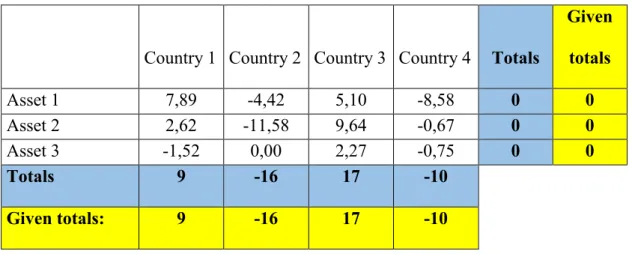
Fortunately, in our more than 25-year experience, we found that the additive- RAS method and the modified additive-RAS method mostly converge fast and usually the resulting matrix fits well to the reference matrix. To illustrate this, we present not one of our exercises but we test it with the numerical example of Huang et al (2008) instead.
29
The numerical test confirmed that the additive-RAS algorithm produces the same result as what Huang et al (2008) published as optimal solution of the INSD-model, which they had found to be the estimation method with the best fit in terms of the AIL (average information loss) measure (which was computed to be 11,28).
In addition, if we follow Temurshoev et al’s (2011) interpretation (or clarification) of the iteration method suggested by Huang et al (2008) it is easy to prove that in the case of the not enforced sign-preserving case, our and their iteration algorithms are the same too. Concretely, while Huang et al (2008) only say that “By initializing α, λ, τ as I, 0, 0 respectively and calculating them with equations (24), (28) and (29) iteratively, we obtain the final solution” where the α stands for the matrix of our zi,j ‘cell indices’ (i.e is the matrix of the ratios of the corresponding elements of the resulting and reference matrices) and where their equations (24), (28) and (29) correspond to our equations (8), (8a) and (8b) respectively, Temurshoev et al (2011) not only correct this by saying that α is (not square but) the m x n matrix of ones, but also say that within each iteration steps λ has to be computed first and only then τ is computed already using the just computed values of λ, while α has to be computed at last. This we call the recursive interpretation of the algorithm suggested by Huang et al (2008) as opposed to the other legitimate interpretation which may be called the contraction-like algorithm in which the iterating variables (vectorised and grouped together in the say w vector) change simultaneously according to the w(n+1) = f (w(n)) symbolic scheme, where f is the operator of the iteration steps.
In the case of the not enforced (but still) sign-preserving case the first step of the Huang et al (2008) suggested iteration algorithm interpreted as contraction-like algorithm are identical to equations (13) and (14). In the recursive interpretation – using equation (10) – equation (14) is replaced by the