Article
Robust Scheduling of Waste Wood Processing Plants with Uncertain Delivery Sources and Quality
Balázs Dávid1,2 , Olivér ˝Osz3 and Máté Hegyháti3,4,*
Citation: Dávid, B.; ˝Osz, O.;
Hegyháti, M. Robust Scheduling of Waste Wood Processing Plants with Uncertain Delivery Sources and Quality.Sustainability2021,13, 5007.
https://doi.org/10.3390/su13095007
Academic Editors: Dragan Pamucar and Željko Stevi´c
Received: 11 April 2021 Accepted: 28 April 2021 Published: 29 April 2021
Publisher’s Note:MDPI stays neutral with regard to jurisdictional claims in published maps and institutional affil- iations.
Copyright: © 2021 by the authors.
Licensee MDPI, Basel, Switzerland.
This article is an open access article distributed under the terms and conditions of the Creative Commons Attribution (CC BY) license (https://
creativecommons.org/licenses/by/
4.0/).
1 InnoRenew CoE, 6310 Izola, Slovenia; balazs.david@innorenew.eu or balazs.david@famnit.upr.si
2 Department of Information Sciences and Technologies, University of Primorska, 6000 Koper, Slovenia;
3 Department of Information Technology, Széchenyi István University, Széchenyi István University, 9026 Gy˝or, Hungary; osz.oliver@sze.hu
4 Institute of Informatics and Mathematics, University of Sopron, 9400 Sopron, Hungary
* Correspondence: hegyhati@sze.hu or hegyhati.mate@uni-sopron.hu
Abstract: While the study of reverse wood value chains has become an important topic recently, optimization-focused studies usually consider network-level problems and decisions, and do not address the individual processes in the network. In the case of waste wood, one such important process is the scheduling of the various machines in a waste wood processing facility to treat incoming wood deliveries with multiple sources and varying quality. This paper proposes a robust multi- objective mixed-integer linear programming model for the optimization of this process that considers the uncertain origins and compositions of the incoming deliveries, while aiming to minimize both lateness and energy consumption. An exhaustive study is performed on instance sets of different sizes and structures to show the efficiency and the limits of the proposed model both in single- and multi-objective cases.
Keywords:reverse wood value chain; scheduling; waste-wood processing
1. Introduction
The topics of recycling and reuse are getting an increased recognition due to the growing importance of sustainability and environmental consciousness. Adding values to residues and wastes not only helps industries meet their commitments towards various EU- and country-level regulations, but also provides an environmentally friendly alternative to other, more traditional resource streams. Still, biomass wastes are mainly considered for energy production [1], which leads to scientific studies of biomass value chains concen- trating mostly on efficient use for energy as well [2]. However, there are certain biomass types where viable alternative uses also exist. Waste wood is a good example for this: it is a versatile material that can be reused and recycled after its original function becomes obsolete, offering a more sustainable option than energy production [3].
Reverse logistics is the field that considers the logistics network of return product flows, putting an emphasis on the end-of-life recovery and the reuse of resources [4].
The three major processes of a reverse logistics network are distribution, production planning and inventory management [5]. Naturally, this may change or become more specialized for certain industrial fields. While the processes remain the same for biomass supply chains, extra emphasis should be put on processing, conditioning and intermediate production, as these can influence the attributes of the transported, stored and utilized biomass products [6]. However, the majority of papers in literature only study inventory and product return management and network design [7], and the optimization of produc- tion processes is rarely considered. This is especially true for waste wood value chains.
While the traditional forward resource flows of wood are well-studied [8,9] and facility- level processes like sawmilling [10] or cutting pattern optimization [11] are also considered, the available literature on the reverse logistics processes of waste wood is significantly
Sustainability2021,13, 5007. https://doi.org/10.3390/su13095007 https://www.mdpi.com/journal/sustainability
scarcer. Apart from studies about the use of waste wood for energy [12,13], the few existing papers revolve around variations of network design [14–17], but the optimization problems arising in the facilities of these networks are not addressed.
This paper studies the arising scheduling problems in a waste wood processing facility over a planning horizon, and presents an optimization approach for their solution.
These facilities are considered as an integral and intermediate process of a waste wood reverse logistics network where various types of wood waste are first collected from the available sources of the network, then transported to such a facility for processing, and finally delivered to customers to satisfy their demands. The wood deliveries arriving to a facility go through a series of transformation processes, and the resulting product is then transported to the customer in its required form. As the incoming deliveries to such a facility can have different origins (e.g., building/industrial or household waste) and characteristics (e.g., coated or uncoated) [18], the exact processing steps that have to be taken might vary between deliveries based on these features. Because of these characteristics, there is an uncertain element to the problem that also has to be taken into account during optimization. Moreover, each delivery has a priority and a deadline that also have to be considered during scheduling.
A mixed-integer linear programming model (MILP) is presented for scheduling the wood deliveries on the various machines of the processing facility in the required order over a fixed planning horizon of several days/weeks. The model considers the robustness of the problem by taking into account the uncertainty that arises because of the varying delivery sources and quality. Optimization is done using two different objective functions;
either ensuring timely completion of the deliveries by considering their priority-weighted lateness, or minimizing the energy consumption of the available machines at the facility.
This allows the generation of different solutions for the same problem scenario using multi-objective optimization, which can aid the decision-making process of production planning at the facility.
The efficiency of the model is presented on input instances of varying sizes and structures. As the acquisition of accurate and exact real-world data is difficult on this level of a supply chain, these instances are randomly generated. The characteristics (origin and type) of incoming deliveries are determined based on real-world distributions published in the literature, while the available machines of the facility have the characteristics of actual existing waste wood processing machinery.
The outline of this paper is the following. First, the arising scheduling problem is defined in detail, describing all constraints that are be taken into account, and a multi- objective MILP model is formalized for the optimization of this problem. Then, the results of this model are presented on various input instances, showing its capabilities and limits.
Finally, the paper is concluded with the presentation of future extension possibilities of the current work.
2. Problem Definition
2.1. General Process and Infrastructure
The approach proposed in this paper tackles the mid-term scheduling of stochastic jobs in a waste wood processing facility. The time horizon of interest spans over several days, starting from the earliest delivery of input materials until the latest deadline. For the scope of this study, time frames of one and two weeks were both examined.
The processing facility receives waste wood deliveries from various sources and has to produce shredded wood out of them by pre-determined deadlines. The production process of a delivery will be referred to as a job. There is a one-to-one relation between jobs and deliveries, thus the two terms will often be used interchangeably.
Incoming waste wood deliveries are categorized according to the information in [18].
Deliveries can belong to multiple categories based on their origin: construction waste, industrial waste, household waste, and waste from collection centers. Due to their similar characteristics, construction and industrials wastes will be merged under the same category
for the remainder of this paper. The same will be true for wastes from households and collection centers. Waste wood of the former category usually arrives directly from the sites, while the latter can come either directly from households or regional collections centers. Independently of their origin, deliveries can also be categorized by the type of the delivered material: they consist of either solid wood or derived timber products.
A key feature of a delivery is the possibility and percentage of contaminations. On top of the above characteristics, a part of each delivery is coated wood that has to go through a removal process. The ratio of coated wood in a delivery depends on its other features.
Derived timber products from households or collection centers are coated in the majority of the cases, while this is not true for industrial and building waste, which is only partly coated. A more detailed classification of deliveries would be possible, however, from the aspect of the current investigation, jobs sharing the same delivery category are assumed to have similar properties. Furthermore, collecting accurate real-world data for finer classification may be practically infeasible.
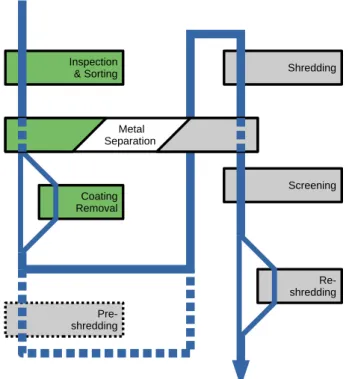
The processing of each job consists of six or seven steps. Five of these steps, in process- ing order, are: inspection, coating removal, shredding, screening, and re-shredding. The sixth step, metal separation can be done either manually between inspection and coating removal, or in an automated fashion by a (magnetic) separator after shredding. For solid wood deliveries from industrial sites, a seventh step, pre-shredding is also required to make the materials suitable for the shredding equipment. The interconnection of the above processes can be seen in Figure1.
Figure 1.The possible flow of waste wood through the different transformation processes (green:
manual steps, gray: machine steps).
In Figure1, each box corresponds to one of the processing steps of the facility, while the blue line represents the flow of the materials. The green-colored steps must be carried out by dedicated crews, gray-colored steps are performed by machines. Coating removal is performed only for the coated part of each delivery, while pre-shredding is only done for solid industrial wood deliveries. The two metal separation steps have a mutually excluding relation: exactly one of them has to be included in the transformation process of every delivery. Similarly to coating removal, re-shredding is only performed on a portion of all materials.
The facility has two types of resources to carry out these tasks. Shredding, pre- shredding, automated metal separation, screening, and re-shredding is done by high-value machines with limited availability. There is no overlap among the machines suitable for these steps, except for shredding and re-shredding, which use the same machines. The rest of the tasks, i.e., inspection, coating removal, and manual metal separation are carried out by dedicated crews. Both machines and the crews have an estimated processing speed, expressed in the processed mass over time. Several suitable machines may be assigned to work in parallel on the same delivery. However, the processing steps are non-preemptive:
they may not be interrupted and resumed later on the same machine. The only interruption occurs at the end of shifts, and the next day processing continues with the same job.
It is assumed that setup and shutdown operations are done before and after the shifts, respectively. Specialized crews for inspection and removal tasks work on a single job at a time, and—similarly to machines—do not switch to other jobs until they are finished with the current one.
While the paper considers shredded wood as the end-product produced by the facility, different wood processing techniques can also be handled in a similar fashion. The pro- posed modeling and solution methodology is flexible enough to accommodate different processes as well, as long as their relations can be defined in a similar way.
2.2. Uncertainty and Objective
The uncertainty of the problem comes from two steps: coating removal and re- shredding. The percentage of coated raw material is not known in advance, it is determined during the inspection step. Similarly, the amount of shredded material, that is not fine enough and requires re-shredding is only revealed during screening. There is, however, statistical data available for both of these for each of the four categories. Since the out- come of the inspection/screening influences the amount of raw material needing coating removal/re-shredding, the time required for these steps is stochastic.
Unless the worst-case scenario is considered for all of the deliveries, the feasibility (i.e., adhering to the deadlines) of a schedule cannot be ensured. However, if processing plans were tailored for the worst-case scenario, the real-life operation would have too much idle time and an oversized machine capacity would be required.
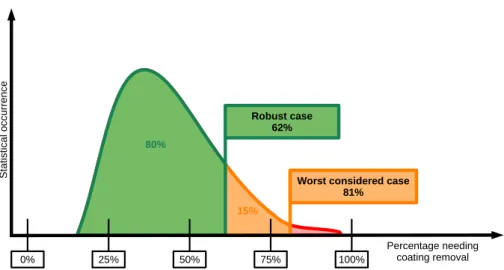
Thus, a different approach and objective is proposed. Two scenarios are modeled simultaneously: worst considered case, and robust case. The theoretical worst case would be when 100% of a delivery requires both coating removal and re-shredding. The probabil- ity of this is very low. Instead of this, the worst considered case assumes ratios needing coating removal and re-shredding, such that the probability that the actual ratios will be lower, is 95%. Similarly, the robust case assumes ratios that are higher or equal to the actual ratios 80% of the time, based on the statistics. These percentages can be set to different values by the experts responsible for daily operation planning, to manage the robustness of the solution.
The cumulative probabilities can be translated into material ratios, based on the probability density functions constructed by estimating the distribution from statistical data. Figure2shows such a probability density function for coating removal. Aiming for 95% and 80% probabilities, this translates to 81%, and 62% of materials needing coating removal in the worst considered and robust cases, respectively. A separate function is created for each delivery category, and for both coating removal and re-shredding.
By fixing uncertain parameters to constant values in each scenario, the same modeling techniques can be applied as in deterministic scheduling problems. Robustness can be specified through the chosen probability values, and more scenarios can be analyzed by rerunning the solution procedure with different values. A possible future research topic is to incorporate uncertainty into the scheduling model in the form of stochastic variables, fuzzy numbers, or by other techniques.
Figure 2.Probability density function for the ratio of raw material needing coating removal based on statistical data.
Scheduling decisions are the same for both scenarios but some constraints and objec- tives are only connected to one of them.
Delivery deadlines impose hard constraints for the robust case. So a schedule is only feasible if no lateness occurs in this scenario. It is important to note that even if some ratios turn out to be over the specified robust threshold, deadlines may still be satisfied due to reserve machine times, which are either inherently present in the schedule, or resulted from lower ratios for other jobs.
For given robustness thresholds, plenty of schedules may be feasible. To select the best of them, two different objectives are proposed in this paper.
The first objective is to minimize deadline violations for the worst considered case.
Deliveries may have different associated penalties, liquidated damages, or importance based on the client. These factors are modeled via a scalar priority, and the exact objective is the priority-weighted sum of lateness. Simply put, the reported solution will be a robust schedule with the lowest possible penalty in the worst case.
Processing machines require a huge amount of electricity to operate. Machine assign- ment to jobs can influence the total energy consumption of the facility, and as a result, its environmental footprint. The second objective is to provide a robust schedule that minimizes this footprint, coming from the energy needs of setup, shutdown, and operation of the machines. Energy need for setup and shutdown is provided for each machine as is.
For operation, two different power values are given per machine: working and idle power.
It is assumed that machines are turned off for the night, and only turned off before the shifts end, if they are not required later on the same day.
2.3. Formal Problem Definition
The proposed problem class can be defined formally by the sets and parameters listed below.
2.3.1. Job Related Data
J is the finite set of jobs/deliveries.
JB,JH are the sets of jobs with building/industrial and household deliveries, respectively.
JB∩JH =∅andJB∪JH= J
JS,JD are the sets of jobs with solid and derived wood deliveries, respectively. JS∩JD =∅ andJS∪JD =J
daj ∈Z0,+is the day of arrival of the delivery for jobj∈ J.[day] dsj ∈Z0,+is the day of shipping of the product for jobj∈J.[day] pj ∈R0,+is the priority of jobj∈J.[−]
mj ∈R0,+is the total mass of the delivery for jobj∈J.[t] 2.3.2. Infrastructure Related Data
cIS,cCR,cMS ∈R0,+ are the throughput capacities for inspection and separation, coating removal, and manual metal separation at the facility, respectively.[t/h]
M is the finite set of machines, the union of the following pairwise disjoint sets:
MMS is the finite set of machines for automated metal separation.
MPS is the finite set of machines for pre-shredding.
MSH= MRS is the finite set of machines for shredding and re-shredding.
MSC is the finite set of machines for screening.
cm,j ∈R0,+is the throughput capacity of a machinem∈Mfor jobj∈ J.[t/h] em ∈R0,+is the electrical power consumption of a machinem∈ M.[kW]
wm ∈R0,+is the total amount of electrical energy needed to shutdown and then start up machinem∈M.[kWh]
s ∈R0,+is the length of the shifts.[h] 2.3.3. Uncertain Data
pCRX,Y,pRSX,Y ∈[0, 1]are the percentages requiring coating removal and re-shredding for jobs with originsX∈ {B,H}and material typeY∈ {S,D}in the robust case.[−]
¯
pCRX,Y,p¯RSX,Y ∈[0, 1]are the percentages requiring coating removal and re-shredding for jobs with originsX∈ {B,H}and material typeY∈ {S,D}in the worst-case scenario.[−]
3. Proposed Approach
In this section we propose a family of Mixed-Integer Linear Programming (MILP) models to tackle the aforementioned optimization problem. All of these models rely on the same basis, and differ in objective functions and/or several constraints. The models can be applied in various ways, as illustrated in Section4: solving them provides the globally optimal solution, or for large problem instances, they may report a close-optimal solution within a short amount of time. Having two objective functions, one can derive a Pareto-curve with iterative execution of the optimizer. The models are developed for offline scheduling, however, by fixing variables that represent already applied decisions, the models may be used in a reactive fashion as well.
The operation of the facility is not continuous,srepresents the total length of work shifts on a day. However, since tasks can be interrupted at the end of shifts and resumed the next day, the active time of the facility can be considered as a continuous time horizon. If something happens at timet≥0 in the model described below, it refers to thet−s· btsc-th hour on thedtse-th day.
3.1. General Structure and Derived Sets
As detailed later, the model follows a precedence-based representation of scheduling decisions. To ease the formulation, several sets are derived from the input data.
As already used for thec,pand ¯pparameters and theMsets above, the following symbolic names represent the processing steps:
IS Inspection and separation CR Coating removal
MS Metal separation PS Pre-shredding SH Shredding RS Re-shredding
SC Screening
Various subsets of these will be used for simpler formalization of the model:
SC ={IS,CR,MS} (1)
SM ={MS,PS,SH,RS,SC} (2)
S=SC∪SM (3)
S¯={CR,RS} (4)
SC contains the steps that could be done manually by dedicated crews, whileSM contains the steps that can be carried out by machines.Sis simply the set of all step types, and ¯Scontains the steps with uncertain load.
The mandatory precedence relations between these steps are stored as pairs in the Pset:
P={(IS,CR),(CR,PS),(CR,SH),(PS,SH),(SH,SC),(SC,RS)} (5) A key derived set for the formulation isT, the set of all processing steps for all jobs, which will be called the set of tasks and can formally be defined as:
T=(j,s)∈ J×S|s6=PS∨j∈ JB∩JS (6) Another useful derived set is the set of possible machine-task assignments:
A=((j,s),m)∈T×M|s∈SM∧m∈ Ms (7) 3.2. Basic Scheduling Variables
As mentioned before, the model follows a precedence based logic. Each task is assigned two non-negative continuous variables indicating its start and completion time:
tsj,s,tcj,s∈[s·daj,s·dsj] ∀(j,s)∈T (8) The decision whether to do metal separation manually or by a machine is represented by the following binary variable:
dj∈ {0, 1} ∀j∈ J (9)
dj =1 means manual separation, anddj=0 represents separation by machines.
Binary variables represent assignment decisions as well, 1 referring to a machine assigned to a task, and 0 if it is not:
aj,s,m∈ {0, 1} ∀((j,s),m)∈A (10)
As parallel execution is allowed, and several machines may be assigned to the same task (e.g., shredding of a single delivery is performed on two or more machines), a continu- ous variable represents the quantity distribution for each assignment:
qj,s,m∈[0,mj] ∀((j,s),m)∈ A (11)
There are tasks that may share one or more machines (e.g., shredding is done on the same machine for two different deliveries). The set of these (ordered) task pairs is given in the following set:
CM=((j1,s1),(j2,s2))∈ T×T|s1,s2∈SM∧Ms1∩Ms2 6=∅∧(j1,s1)6= (j2,s2) (12) Note, that as most steps have their separate machines,s16=s2only occurs, if one of them isSHand the other isRS.
If such tasks are both assigned to at least one shared machine, they have to be sequenced.
The following variable takes the value of 1, if(j1,s1)must precede(j2,s2)if at least one shared machine is assigned to both of them. The value 0 indicates the opposite direction.
bMj1,s1,j2,s2 ∈ {0, 1} ∀((j1,s1),(j2,s2))∈A (13) For manual jobs, each step has a dedicated crew, and thus assignment collision is there for all job pairs. A similar set toCMis defined for manual jobs, however, in this case it only contains triplets, as the step has to be the same for colliding tasks:
CC=(j1,s,j2)∈J×SC×J|j16=j2 (14) And a similar binary variable represents sequencing:
bCj1,s,j2 ∈ {0, 1} ∀(j1,s,j2)∈CC (15) Finally,Mwill denote a sufficiently large number for relaxations in big-M constraints.
3.3. Constraints
3.3.1. Logical and Balance Constraints
There are some logical dependencies between the decisions represented by the intro- duced binary variables, that can be expressed by the following constraints.
aj,MS,m≤1−dj ∀((j,MS),m)∈A (16)
bCj1,s,j2+bCj2,s,j1 =1 ∀(j1,s,j2)∈CC\ {MS} (17) bCj1,MS,j2+bCj2,MS,j1 ≤ dj1+dj2
2 ∀(j1,MS,j2)∈CC (18) bCj1,MS,j2+bCj2,MS,j1 ≥dj1+dj2−1 ∀(j1,MS,j2)∈CC (19) bMj1,s1,j2,s2+bMj2,s2,j1,s1 =1 ∀((j1,s1),(j2,s2))∈CM:s16=MS (20) bMj1,MS,j2,MS+bMj2,MS,j1,MS≤1−dj1+dj2
2 ∀((j1,MS),(j2,MS))∈CM (21) bMj1,MS,j2,MS+bMj2,MS,j1,MS≥1−dj1−dj2 ∀((j1,MS),(j2,MS))∈CM (22) Equation (16) ensures that no machine is assigned to metal separation if it is decided to be done manually. Equation (17) states that for every job pair and manual step, one of the jobs should precede the other for that step. Metal separation is handled sepa- rately in Equations (18) and (19) to address the possibility of automated metal separation.
Equations (20)–(22) do the same for steps carried out by machines, addressingMSsepa- rately again.
(j,s,m)∈A
∑
qj,s,m=mj ∀(j,s)∈T:s∈ {PS,SH,SC} (23)
(j,MS,m)∈A
∑
qj,MS,m=mj·(1−dj) ∀j∈ J (24)
(j,RS,m)∈A
∑
qj,s,m=pRSX,Y·mj ∀X∈ {B,H},Y∈ {S,D},j∈ JX∩JY (25)
qj,s,m≤mj·aj,s,m ∀((j,s),m)∈ A (26)
Equations (23)–(25) enforce that the sum of the quantities assigned to machines at a step should add up to the total load. Besides metal separation, re-shredding needs a separate constraint as well, due to its uncertain nature. Equation (26) allows only assigned units to process a non-zero quantity for a task.
3.3.2. Processing Time Constraints
The following constraints set the relation between the starting and completion times of tasks.
tcj,IS=tsj,IS+ mj
cIS ∀j∈ J (27)
tcj,MS≥tsj,MS+ mj
cMS−M·(1−dj) ∀j∈J (28) tcj,MS≤tsj,MS+ mj
cMS+M·(1−dj) ∀j∈J (29) tcj,CR=tsj,CR+pCRX,Y· mj
cCR ∀X∈ {B,H},Y∈ {S,D},j∈ JX∩JY (30) tcj,s,c≥tsj,s,c+ qj,s,m
cm,j ∀((j,s),m)∈ A (31) Inspection and separation is the simplest to address (27), metal separation needs special attention due to possible automated execution (28), and coating removal has its own equation as well due to its uncertain nature (30).
A single constraint, Equation (31) sets the difference between completion and starting time for all tasks that are carried out by machines.
3.3.3. Production Precedence Constraints
The following 5 equations express mandatory production sequencing due to mate- rial flows.
tsj,sn ≥tcj,sp ∀j∈ J,(sp,sn)∈ P:(j,sp)∈T∧(j,sn)∈T (32) Equation (32) enforces all mandatory production precedence relations inPfor all jobs.
Namely, ifspis a predecessor step ofsn, then the starting time ofsnmust be at earliest the completion time ofsp.
tsj,MS≥tcj,IS−M·(1−dj) ∀j∈ J (33) tsj,CR≥tcj,MS−M·(1−dj) ∀j∈ J (34) tsj,MS≥tcj,SH−M·dj ∀j∈ J (35) tsj,SC≥tcj,MS−M·dj ∀j∈ J (36) Equations (33) and (34) handle the case when metal separation is done by a ded- icated crew, and it must be carried out after inspection and before coating removal.
Equations (35) and (36) address the other case, when the metal separation is done by a machine, then it must follow shredding and precede screening.
3.3.4. Scheduling Precedence Constraints
The following two constraints express timing constraints that are the results of se- quencing decisions made bybCandbMbinary variables.
tsj2,s ≥tcj
1,s−M·(1−bCj1,s,j2) ∀(j1,s,j2)∈CC (37)
tsj2,s2 ≥tcj1,s1−M·(3−aj1,s1,m−aj2,s2,m−bMj1,s1,j2,s2)
∀((j1,s1),(j2,s2))∈CM,m∈Ms1∩Ms2 (38) Equation (37) handles sequencing of dedicated crews, while Equation (38) addresses machine sequencing.
3.4. Objective Functions
As discussed before, two different objective functions are considered here, and each requires additional variables and constraints to be calculated. Most of these variables are
fixed or computed, e.g., they do not introduce additional decisions into the model, rather they are the consequences of the decisions made by the preexisting variables.
3.4.1. Priority Weighted Lateness Minimization
As this objective function intends to minimize the total weighted lateness in the worst considered case, an alternate timing for each task needs to be calculated. In order to achieve that, a worst considered scenario versions ofts,tcandqvariables need to be defined over the same domains: ¯ts, ¯tc, and ¯q. The only difference is that the upper limit of ¯ts and ¯tc is infinity instead ofs·dsj. These variables represent the starting and completion times, and the load of machines when coating removal and re-shredding takes longer in the worst considered case.
To set these variables, Equations (23)–(38) need to be duplicated with the worst considered case variables instead of the robust case ones.
An additional set of continuous variables, the number of late days of each job needs to be introduced:
l¯j ∈Z0,+ ∀j∈ J (39)
Equation (40) calculates the values for these variables:
t¯cj,RS≤(dsj+l¯j)·s ∀j∈J (40) Then, the objective function can be defined as:
∑
j∈Jpj·l¯j→min (41)
3.4.2. Electrical Footprint Minimization
To ease the formulation of this objective function, a set for the considered days (in the robust case) is defined as:
Hj ={daj−1, . . . ,dsj+1} ∀j∈ J (42)
H=∪j∈JHj (43)
An additional binary variable is introduced to indicate whether a machine is turned on or not on a particular day:
um,d∈ {0, 1} ∀m∈ M,d∈H (44)
The total energy consumption is the sum of electricity used for processing tasks and the energy used to start up and shut down machines on active days. This objective can be expressed as:
(j,s,m)∈A
∑
qj,s,m·em
cm,j +
∑
m∈M,d∈H
um,d·wm→min (45)
However,uneeds to be computed fromtandavariables. In order to do that, an auxil- iary computed binary variable is introduced to indicate if a machine works on a task at a given day:
yj,s,m,d∈ {0, 1} ((j,s),m)∈ A,d∈ Hj (46)
If a machine works on at least one task on a day, it must be turned on, as expressed by Equation (47):
um,d≥yj,s,m,d ∀((j,s),m)∈ A,d∈ Hj (47)
A machine must work on a task at least as many days as many is needed to process the assigned quantity:
d∈H
∑
yj,s,m,d≥ qj,s,m
cm,j·s ∀((j,s),m)∈A (48) The following constraints ensure that a task does not start on an earlier day or end on a later one than indicated by the correspondingyvariables:
tsj,s ≥d·s−M·(1−yj,s,m,d+yj,s,m,d−1) ∀((j,s),m)∈ A,d∈ Hj:d>daj (49) tcj,s ≤(d+1)·s+M·(1−yj,s,m,d+yj,s,m,d+1) ∀((j,s),m)∈A,d∈Hj :d<dsj (50) tsj,s ≤(d+1)·s+M·(1−yj,s,m,d) ∀((j,s),m)∈ A,d∈ Hj:d≥dsj (51) tcj,s ≥d·s−M·(1−yj,s,m,d) ∀((j,s),m)∈ A,d∈Hj :d≤dsj (52) 3.5. Overview of the Mathematical Model
A structural overview of the sets, parameters, and variables used in the proposed model is illustrated in Table1. The table details the sets and parameters that are provided as input data, and the ones that are derived from others. Moreover, it also highlights the parameters, sets, and variables that are required for the base model or one of the objective functions.
Table 1.Overview of model notations.
BASE MODEL
Input data sets JB,JH,JS,JD,MMS,MPS,MSH,MSC parameters daj,dsj,mj,cIS,cCR,cMS,cm,j,s,pCRX,Y,pRSX,Y Derived sets J,M,MRS,SC,SM,S, ¯S,P,T,A,CM,CC Decision variables continuous tsj,s,tcj,s,qj,s,m
binary dj,aj,s,m,bMj
1,s1,j2,s2,bCj
1,s,j2
PRIORITY WEIGHTED LATENESS MINIMIZATION Additional input data pj, ¯pCRX,Y, ¯pRSX,Y
Additional variables continuous t¯sj,s, ¯tcj,s, ¯qj,s,m
discrete l¯j
Objective function ∑j∈Jpj·l¯j
ELECTRICAL FOOTPRINT MINIMIZATION Additional input data Hj,H,em,wm
Additional variables binary um,d,yj,s,m,d
Objective function ∑(j,s,m)∈A
qj,s,m·em
cm,j +∑m∈M,d∈Hum,d·wm
4. Numerical Results
In order to properly test the efficiency of the proposed model, a large number of tests had to be carried out on instances of varying sizes and structures. While acquiring single instances can be manageable by monitoring a collection center over a given period, solving only a handful of these does not show the general usefulness of the model, rather its functionality on a couple of dedicated use-cases. Existing large-scale information about waste generation, collection and processing is mostly published as statistical data, aggregated usually in a yearly fashion [19]. Such data cannot be decomposed into actual real-life scenarios, but information about the general structure of real-world instances can be derived from them. Because of this limitation, instances used for testing the model were randomly generated based on studies about the characteristics and distributions of
wood waste. Randomly generated instances can turn out to be infeasible, usually in cases where a greater amount of deliveries arriving around the same time cannot be processed by their given deadline due to the limited capacity of the available machines. However, such inputs are also useful for testing purposes to see how efficiently infeasibility can be reported. Proving the infeasibility of scenarios is not always a trivial task, but it should be within the capabilities of the model.
Features of the deliveries such as their origin (building or industrial waste, and wastes from households and collection centers) and type (solid or derived) were determined based on statistics in [18]. While that study discusses the four origins independently of each other, we merged them into two groups based on their similarities for the sake of simplicity and easier presentation. Naturally, the model would function the same way with four different origins.
The total mass of deliveries was determined based on the potential payloads of biomass transport trucks [20]. Two different payload ranges were considered. Instances with a small payload contained deliveries of 19–23 t, that could hypothetically be processed on their arrival day, while the deliveries of instances with large, 31–49 t payloads could take more than one day to process. Information of the machines (throughput and energy use) for the different tasks was based on real machinery [21]. Three machines with differ- ent properties were available for every machine task, each extra option offering higher throughput in exchange for more energy use. Only a single crew was provided for each manual step of the process, and their throughput was intentionally set significantly lower than that of the machine steps. This resulted in inspection and sorting being the bottleneck of the scheduling process, as every delivery had to go through this step, and there are no machine alternatives for it. For this reason, tests were run both with the original 10 t/h throughput, and with doubling this efficiency.
A large number of tests were performed with optimizing for either one of the objective functions, or solving the combined bi-objective optimization problem. The proposed model was solved using Gurobi 9.1 solver for every instance. Tests were run on a PC with an Intel Core i7-5820K 3.30 GHz CPU and 32 GB memory.
4.1. Single Objective Optimization
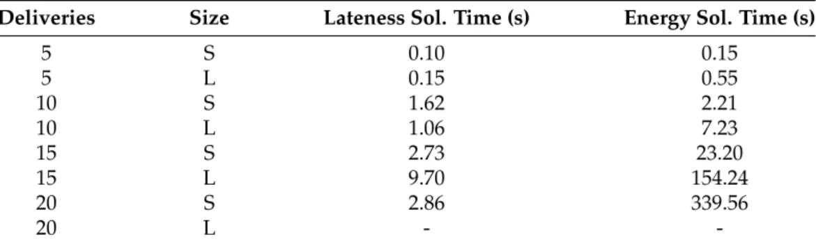
The first set of input instances were generated over a one-week horizon. The arrival day of the deliveries was chosen in a uniformly random way from this period, and the deadlines were also uniformly random: 1–2 days from arrival for small deliveries and 2–3 days for large deliveries. Various instance sets were generated with delivery numbers between 5 and 20, and the average running times of instances of the same set are presented in Table2for the slower inspection throughput, and Table3for the faster one. Each row of the tables gives the number of deliveries and delivery size (S—small, L—large) of the instances group, and provides an average optimization time for a set of 10 randomized instances in the case of minimizing their lateness or energy use. The optimization time corresponds to the time needed to either achieve an optimal solution or determine the infeasibility of the instance under the current parameter settings. A running time limit of one hour (3600 s) was enforced on the solution process. In some cases, non-optimal solutions were found within the time limit, these will be explained in detail when discussing the corresponding tables. Such occurrences are marked with an * next to the average running time.
In the case of the one-week horizon and a slower inspection throughput, the running time limit was reached for two inputs of the (15,L) instance set while minimizing energy use. The instances were infeasible in both cases. However, this infeasibility was found in under 10 s when optimizing for minimal lateness, so these running times were used when calculating the energy use average. Results for the (20,L) instances are not provided, as they were infeasible in every case, because the planning horizon was too small to schedule every delivery on the available machines.
Table 2.Average results of a one-week horizon and slower inspection and sorting process.
Deliveries Size Lateness Sol. Time (s) Energy Sol. Time (s)
5 S 0.10 0.15
5 L 0.15 0.55
10 S 1.62 2.21
10 L 1.06 7.23
15 S 2.73 23.20
15 L 9.70 154.24
20 S 2.86 339.56
20 L - -
Doubling the speed of the inspection and sorting step shows a more efficient solution process, the results of which are presented in Table3.
Table 3.Average results of a one-week horizon and faster inspection and sorting process.
Deliveries Size Lateness Sol. Time (s) Energy Sol. Time (s)
5 S 0.09 0.13
5 L 0.13 0.49
10 S 0.30 0.46
10 L 0.54 8.62
15 S 1.46 5.35
15 L 38.36 743.70
20 S 7.45 86.17
20 L 979.11 * 1243.16 *
Optimal solutions were found for all instances for the sizes of 5, 10 and 15 deliveries except for one: in the (15,L) instance set, a single solution reached the time limit, and pro- duced a non-optimal result with a 2.18% gap. However, while solutions were found for all instances of the (20,L) instance set, only 5 were optimal when optimizing for lateness, and 7 were optimal when optimizing for energy. The suboptimal solutions found for the remaining instances had a greater than 50% optimality gap in every case. As a result, these are not considered in the averages of Table3. As bad-quality suboptimal solutions were found for multiple inputs in this (20,L) instance set, this seems to be the limit of the model considering the given time limit. Efficient (optimal, or close-to-optimal) solutions were found for all other problem classes with a short average running time.
The model was tested for larger delivery numbers as well. However, as slower inspection resulted in infeasible solutions for the (20,L) instances, these larger inputs were tested over a two-week planning horizon. The instance sets were generated under the same conditions as the one-week sets. Their average running times can be seen in Table4in the case of slower inspection throughput, and Table5in the faster case.
Table 4.Average results of a two-week horizon and slower inspection and sorting process.
Deliveries Size Lateness Sol. Time (s) Energy Sol. Time (s)
20 S 3.59 72.37
20 L 21.59 * 494.32 *
25 S 10.02 113.25
25 L 431.46 * 1655.49 *
30 S 17.23 * 549.61 *
30 L - -
When using the slower throughput for inspection and sorting, two instances in the (20,L) set did not yield any result in the one hour limit when optimizing for energy.
However, these instances were shown to be infeasible under 60 s when optimizing for lateness, so these values were used for calculating the average runtime. Another instance did not provide an optimal solution in one hour, and the best feasible solution had a 3.79% gap. The (25,L) set had one instance where no optimal solution was found for either objective function in an hour, but the optimality gap of the best solution was 83.88% and 17.29% respectively. Another three instances only gave optimal solutions for minimizing lateness, but could only find near-optimal solutions for minimizing energy with 3.65%, 5.69% and 2.57% gaps. One such instance was also present for (30,S), where only a solution with a 2.33% gap was found in one hour. Two inputs of this set did not yield any results in the one hour running time limit for either objective function. These inputs were not considered in the averages. Minimizing lateness for the same instances yielded an optimal result below 60 s. The instances of the (30,L) set, however, were either all infeasible, of no solution was found in the one hour limit, so their results are not presented in the table.
Again, transitioning to a faster inspection and sorting throughput provides more efficient results, which can be seen in Table5.
Table 5.Average results of a two-week horizon and faster inspection and sorting process.
Deliveries Size Lateness Sol. Time (s) Energy Sol. Time (s)
20 S 1.68 4.80
20 L 9.10 329.92
25 S 5.28 36.56
25 L 144.57 * 2445.34 *
30 S 17.45 776.60
30 L - -
It can be seen from the table that optimal solutions were found for all instances schedul- ing short deliveries regardless of their problem sizes. In the case of the (25,L) instances, time limit was reached for a single input when optimizing for lateness. The suboptimal solution had a 44.06% optimality gap, and it is not included in the average. Time limit was reached in five cases when minimizing energy consumption for the same instance set. However, these solutions were much closer to the optimum (with respective gaps of 4.74%, 1.82%, 5.31%, 2.87% and 0.93%), and their running time was included in the average.
Solution of the (30,L) instance set inputs, however, reached the time limit on every occasion, and while solutions were found, their optimality gap was above 50% in every case. This clearly shows that this instance set is not solvable in the given time limit, and results are not presented for this reason.
If the goal is the optimization of a single objective, it can be seen from the above results that the model can efficiently schedule a big number of smaller deliveries over both a one- and two-week horizon, and has no problem with larger deliveries up to a certain problem size. While solutions could not be acquired for some instances in the given time limit, or their quality was not good enough, this can be remedied with the increase of available running time for the solution process. The solution of the model is significantly easier when optimizing for lateness, which was expected due to the added complexity of the large number of extra binary decision variables in the case of the energy minimization objective.
4.2. Bi-Objective Optimization
In the case of considering both objectives at the same time, a bi-objective optimization problem has to be solved. One option for this is the augmented ε-constraint method introduced in [22]. This method yields multiple non-dominated solutions for the problem, meaning that there is no obvious best solution among them. Such a set of solutions where one cannot find an improved alternative to any of them is called a Pareto front.
The solutions of this front are achieved by solving a series of optimization problems based on the original model. First, the lexicographic method is applied: the objectives are assigned a hierarchical ordering, and the model is solved considering all objectives in this
order. Two hierarchical optimization problems are solved, one having the lateness objective on top of the hierarchy, while the other having the energy objective. Using the objective values of these solutions, the possible value range can be determined for each objective.
This value range is then divided along multiple grid points, and an optimization problem is solved for every region of this division. The number of problems to be solved depends on the chosen number of grid points, which acts as a parameter of theε-constraint method.
UsingGgrid points will result inG+1 regions.
Based on the experiences from the single objective cases, bi-objective optimization was carried out for problem sizes of 5–25 deliveries. Inputs with 5–15 deliveries were generated over a one-week horizon, while inputs with 20 and 25 deliveries were generated over a two- week horizon. For each delivery number, 10-10 instances were generated with small and large deliveries. Bi-objective optimization was carried out for all of these instances using both 5 and 10 grid points, resulting in 6 or 11 problems to be solved. A time limit of 30 min (1800 s) was set for the individual solution processes. Instance sets were generated with both slower and faster inspection and sorting throughput similarly to the single-objective case. Aggregated results can be seen in Table6for the slower, and Table7for the faster throughput. Both tables present the number and size of deliveries in the given instance set, as well as the number of instances where the solution process was terminated due to reaching the time limit. For instances where solutions were achieved, the average number of solutions in the Pareto front and the average required solution time is presented both for the 5 and 10 grid point divisions.
Table 6.Average bi-objective results with slower inspection and sorting process.
Deliveries Size Limit Reached Division 5 Division 10 Front Time (s) Front Time (s)
5 S 0 1.20 0.72 1.20 0.89
5 L 0 1.00 1.13 1.00 1.07
10 S 0 1.60 7.43 1.70 11.32
10 L 0 2.10 172.48 2.10 303.07
15 S 0 3.10 46.61 3.20 80.23
15 L 3 3.71 1321.81 3.86 2079.09
20 S 0 3.00 109.42 3.20 181.13
20 L 4 2.50 1331.42 2.67 1981.28
25 S 0 3.10 593.51 3.50 1043.97
25 L 10 - - - -
Table 7.Average bi-objective results with faster inspection and sorting process.
Deliveries Size Limit Reached Division 5 Division 10 Front Time (s) Front Time (s)
5 S 0 1.10 0.62 1.10 0.70
5 L 0 1.00 0.92 1.00 0.90
10 S 0 1.80 12.44 1.80 18.75
10 L 0 1.40 185.86 1.40 316.93
15 S 0 2.60 50.88 2.80 85.67
15 L 4 3.67 2314.70 4.33 3952.80
20 S 0 2.50 75.03 2.60 118.81
20 L 4 3.83 1809.51 4.17 3213.87
25 S 0 3.40 631.90 3.70 896.69
25 L 10 - - - -
In the case of using the slower inspection throughput, the finer division of 10 grid points usually produced the same number of solutions for the front than the 5-grid point
division, or provided at most one additional. However, having 10 grid points leads to an average of 63% increase in running time for the bigger instances. Instances of the (25,L) set were not solvable in the given time limit, and solutions are not presented for them as a result.
Instances with faster inspection throughput behaved similarly to the previous instance sets. The finer 10-grid point division again produced at most one additional solution compared to the 5-grid point division with an average of 64% increase in running time for the bigger instances. There was a notable exception for one instance in the (15,S) set, where the 10-point division resulted in 9 solutions as opposed to the 6 solutions of the 5-point division. Instances of the (25,L) set were not solvable in the given time limit, and their solutions are not presented.
It can be seen from the above tables that efficient bi-objective optimization of the model is also possible. Multiple non-dominated solutions can be found for the problems in an acceptable time. Results show that increasing the size of the division from 5 to 10 grid points usually results in the same number of solutions, or provides only one additional result. However, this comes at the cost of a significant increase in running time. There was only a single instance where the finer division provided three additional solutions to the front.
5. Conclusions
This paper studied the problem of scheduling the machines in a waste wood pro- cessing facility where the incoming deliveries can come from various sources and have uncertain compositions. A multi-objective mixed-integer linear programming model was presented for the problem to provide robust solutions that minimize lateness and en- ergy consumption. The efficiency of the method was shown on instances with various sizes, which were randomly generated based on real-world distribution data. Computa- tional tests showed that the approach can provide mid-term (1–2 weeks) schedules for 25–30 deliveries in under an hour. The bi-objective model allows the consideration of alternative solutions based on both economic and sustainability factors.
The topic has possibilities for future research. In the current model, a simplified energy cost function was considered. The approach can be extended with a more detailed energy model, for example, considering the idle power of machines between tasks during a day, possibly with additional decisions about when to turn them off. Another possible extension is to model different operation profiles for machines, which allow more energy-efficient processing with the expense of slower throughput. To achieve better overall throughput, the scheduling model could be improved to allow overlap between subsequent processing steps. Some extensions can be too computationally intensive to solve with an exact MILP solver, so a metaheuristic solution approach may also be beneficial for future research.
Author Contributions:Conceptualization, B.D., O. ˝O. and M.H.; methodology, B.D., O. ˝O. and M.H.;
software, B.D.; validation, B.D., O. ˝O.; formal analysis, B.D. and M.H.; investigation, B.D.; resources, B.D.; writing—original draft preparation, B.D., O. ˝O. and M.H.; writing—review and editing, B.D., O. ˝O. and M.H.; visualization, M.H. All authors have read and agreed to the published version of the manuscript.
Funding: This research was supported by the National Research, Development and Innovation Office, NKFIH grant no. 129178. Balázs Dávid gratefully acknowledges the European Commission for funding the InnoRenew CoE project (Grant Agreement #739574) under the Horizon2020 Widespread- Teaming program, and the Republic of Slovenia (Investment funding of the Republic of Slovenia and the European Union of the European Regional Development Fund), and he is also grateful for the support of the Slovenian ARRS grant N1-0093. The authors would also like to thank the Slovenian Research Agency (ARRS) for funding infrastructure program IO-0035.
Acknowledgments: Balázs Dávid acknowledges the Slovenian Research Agency (ARRS) for the bilateral project BI-AT/20-21-014. The Authors would like to acknowledge the work of Endre Bodó, who was helping the research with testing the developed method. He was supported by
“Integrated program for training new generation of scientists in the fields of computer science”, no.
EFOP-3.6.3-VEKOP-16-2017-0002 (supported by the European Union and co-funded by the European Social Fund).
Conflicts of Interest:The authors declare no conflict of interest.
References
1. Tripathi, N.; Hills, C.; Singh, R.; Atkinson, C. Biomass waste utilisation in low-carbon products: Harnessing a major potential resource.NPJ Clim. Atmos. Sci.2019,2, 35, doi:10.1038/s41612-019-0093-5.
2. Nunes, L.; Causer, T.; Ciolkosz, D. Biomass for energy: A review on supply chain management models. Renew. Sustain. Energy Rev.2020,120, 109658, doi:10.1016/j.rser.2019.109658.
3. Garcia, C.A.; Hora, G. State-of-the-art of waste wood supply chain in Germany and selected European countries. Waste Manag.
2017,70, 189–197, doi:10.1016/j.wasman.2017.09.025.
4. Dekker, R.; Fleischmann, M.; Inderfurth, K.; Wassenhove, L.N.V. (Eds.) Reverse Logistics; Springer: Berlin/Heidelberg, Germany, 2004; doi:10.1007/978-3-540-24803-3.
5. Salema, M.I.G.; Barbosa-Povoa, A.P.; Novais, A.Q. An optimization model for the design of a capacitated multi-product reverse logistics network with uncertainty. Eur. J. Oper. Res.2007,179, 1063–1077, doi:10.1016/j.ejor.2005.05.032.
6. Fiedler, P.; Lange, M.; Schultze, M. Supply logistics for the industrialized use of biomass—Principles and planning approach. In Proceedings of the 2007 International Symposium on Logistics and Industrial Informatics, Wildau, Germany, 13–15 September 2007; pp. 41–46, doi:10.1109/LINDI.2007.4343510.
7. Kazemi, N.; Modak, N.M.; Govindan, K. A review of reverse logistics and closed loop supply chain management studies published in IJPR: A bibliometric and content analysis.Int. J. Prod. Res.2019,57, 4937–4960, doi:10.1080/00207543.2018.1471244.
8. Troncoso, J.J.; Garrido, R.A. Forestry production and logistics planning: An analysis using mixed-integer programming. For.
Policy Econ.2005,7, 625–633, doi:10.1016/j.forpol.2003.12.002.
9. Kaltenbrunner, M.; Huka, M.A.; Gronalt, M. Adaptive Model Building Framework for Production Planning in the Primary Wood Industry. Forests2020,11, 1256, doi:10.3390/f11121256.
10. Maturana, S.; Pizani, E.; Vera, J. Scheduling production for a sawmill: A comparison of a mathematical model versus a heuristic.
Comput. Ind. Eng.2010,59, 667–674, doi:10.1016/j.cie.2010.07.016.
11. Koch, S.; König, S.; Wäscher, G. Integer linear programming for a cutting problem in the wood-processing industry: A case study.
Int. Trans. Oper. Res.2009,16, 715–726, doi:10.1111/j.1475-3995.2009.00704.x.
12. Greinert, A.; Mrówczy ´nska, M.; Szefner, W. The Use of Waste Biomass from the Wood Industry and Municipal Sources for Energy Production. Sustainability2019,11, 3083, doi:10.3390/su11113083.
13. Marchenko, O.; Solomin, S.; Kozlov, A.; Shamanskiy, V.; Donskoy, I. Economic Efficiency Assessment of Using Wood Waste in Cogeneration Plants with Multi-Stage Gasification. Appl. Sci.2020,10, 7600, doi:10.3390/app10217600.
14. Devjak, S.; Tratnik, M.; Merzelj, F. Model of Optimization of Wood Waste Processing in Slovenia. InOperations Research ’93;
Bachem, A., Derigs, U., Jünger, M., Schrader, R., Eds.; Physica: Heidelberg, Germany, 1994; pp. 103–107.
15. Burnard, M.; Tavzes, ˇC.; Toši´c, A.; Brodnik, A.; Kutnar, A. The Role of Reverse Logistics in Recycling of Wood Products. In Environmental Implications of Recycling and Recycled Products; Springer: Singapore, 2015; pp. 1–30, doi:10.1007/978-981-287-643-0_1.
16. Trochu, J.; Chaabane, A.; Ouhimmou, M. Reverse logistics network redesign under uncertainty for wood waste in the CRD industry. Resour. Conserv. Recycl.2018,128, 32–47, doi:10.1016/j.resconrec.2017.09.011.
17. Egri, P.; Dávid, B.; Kis, T.; Krész, M. Robust Reverse Logistics Network Design. InLogistics Operations and Management for Recycling and Reuse; Golinska-Dawson, P., Ed.; Springer: Berlin/Heidelberg, Germany, 2020; pp. 37–53, doi:10.1007/978-3-642-33857-1_3.
18. Kharazipour, A.; Kües, U. Recycling of Wood Composites and Solid Wood Products. InWood Production, Wood Technology, and Biotechnological Impacts; Universitätsverlag: Göttingen, Germany, 2007; pp. 509–533.
19. Cocchi, M.; Vargas, M.; Tokacova, K. European Wood Waste Statistics Report for Recipient and Model Regions; Technical Report;
Absorbing the Potential of Wood Waste in EU Regions and Industrial Bio-based Ecosystems (BioReg): 2019. Available online:
https://www.bioreg.eu/assets/delivrables/BIOREG%20D1.1%20EU%20Wood%20Waste%20Statistics%20Report.pdf (accessed on 6 April 2021).
20. Laitila, J.; Asikainen, A.; Ranta, T. Cost analysis of transporting forest chips and forest industry by-products with large truck-trailers in Finland. Biomass Bioenergy2016,90, 252–261, doi:10.1016/j.biombioe.2016.04.011.
21. Komptech. Stationary Machines. Available online: https://komptech.ca/wp-content/uploads/2020/09/Komptech-Stationary- Machines_2018_E.pdf(accessed on 6 April 2021).
22. Mavrotas, G. Effective implementation of theε-constraint method in Multi-Objective Mathematical Programming problems.
Appl. Math. Comput.2009,213, 455–465, doi:10.1016/j.amc.2009.03.037.