Strong limit theorems for random fields

(1)

Strong limit theorems for random fields

Allan Gut

Department of Mathematics, Uppsala University, Uppsala, Sweden e-mail: allan.gut@math.uu.se

Dedicated to Mátyás Arató on his eightieth birthday

Abstract

The aim of the present paper is to review some joint work with Ulrich Stadtmüller concerning random field analogs of the classical strong laws.

In the first half we start, as background information, by quoting the law of large numbers and the law of the iterated logarithm for random sequences as well as for random fields, and the law of the single logarithm for sequences.

We close with a one-dimensional LSL pertaining to windows, whose edges expand in an “almost linear fashion”, viz., the length of the nth window equals, for example, n/logn orn/log logn. A sketch of the proof will also be given.

The second part contains some extensions of the LSL to random fields, after which we turn to convergence rates in the law of large numbers. Departing from the now legendary Baum–Katz theorem in 1965, we review a number of results in the multiindex setting. Throughout main emphasis is on the case of “non-equal expansion rates”, viz., the case when the edges along the different directions expand at different rates. Some results when the power weights are replaced by almost exponential weights are also given.

We close with some remarks on martingales and the strong law.

Keywords: i.i.d. random variables, law of large numbers, law of the iterated logarithm, law of the single logarithm, random field, multiindex.

MSC: Primary 60F05, 60F15, 60G70, 60G60; Secondary 60G40.

1. Introduction

LetX, X1, X2, . . . be independent, identically distributed (i.i.d.) random variables with partial sumsSn, n≥ 1, and setS0 = 0. The two most famous strong laws are the Kolmogorov strong law and the Hartman–Wintner Law of the iterated logarithm:

Proceedings of the Conference on Stochastic Models and their Applications Faculty of Informatics, University of Debrecen, Debrecen, Hungary, August 22–24, 2011

125

(2)

Theorem 1.1(The Kolmogorov strong law — LLN). Suppose thatX, X1, X2, . . . are i.i.d. random variables with partial sumsSn, n≥1.

(a) If E|X|<∞andE X =µ, then Sn

n

a.s.→ µ as n→ ∞. (b) If ^S_nⁿ ^a.s.→ c for some constantc, asn→ ∞, then

E|X|<∞ and c=E X.

(c) If E|X|=∞, then

lim sup

n→∞

|Sn|

n = +∞.

Remark 1.2. Strictly speaking, we presuppose in (b) that the limit can only be a constant. That this is indeed the case follows from the Kolmogorov zero–one law.

Considering this, (c) is somewhat more general than (b). For proofs and details, see e.g. Gut (2007), Chapter 6.

Theorem 1.3 (The Hartman–Wintner law of the iterated logarithm — LIL).

Suppose that X, X1, X2, . . . are i.i.d. random variables with mean 0 and finite varianceσ², and setSn=Pn

k=1Xk,n≥1. Then lim sup

n→∞ (lim inf

n→∞) Sn

p2σ²nlog logn = +1 (−1) a.s. (1.1) Conversely, if

P

lim sup

n→∞

|Sn|

√nlog logn <∞

>0, thenE X²<∞,E X= 0, and (1.1) holds.

The sufficiency is due to Hartman and Wintner (1941). The necessity is due to Strassen (1966). For this and more, see e.g. Gut (2007), Chapter 8.

Remark 1.4. The Kolmogorov zero–one law tells us that the limsup is finite with probability zero or one, and, if finite, the limit equals a constant almost surely.

Thus, assuming in the converse that the probability is positive is in reality assuming that it is equal to 1. This remark also applies to (e.g.) Theorem 1.8.

The Kolmogorov strong law, which relates to the first moment, was generalized by Marcinkiewicz and Zygmund (1937) into a result relating to moments of order between 0 and 2; cf. also Gut (2007), Section 6.7:

Theorem 1.5(The Marcinkiewicz–Zygmund strong law). Let0< r <2. Suppose thatX, X1, X2, . . . are i.i.d. random variables. If E|X|^r<∞andE X= 0when 1≤r <2, then

Sn

n^1/r

a.s.→ 0 as n→ ∞ ⇐⇒ E|X|^r<∞ and, if 1≤r <2, E X= 0.

(3)

The results so far pertain to partial sums, summing from X1 and onwards.

There exist, however, analogs pertaining todelayed sums or windows or lag sums, that have not yet reached the same level of attention, most likely because they are more recent.

In order to describe these results we define the concept of awindow, say. Namely for any given sequenceX1, X2, . . . we set

Tn,n+k =

n+kX

j=n+1

Xj, n≥0, k≥1.

The analogs of the strong law large numbers and the law of the iterated logarithm are due to Chow (1973) and Lai (1974), respectively.

Theorem 1.6(Chow’s strong law for delayed sums). Let 0< α <1, suppose that X, X1, X2, . . . are i.i.d. random variables, and set Tn,n+n^α=Pn+n^α

k=n+1Xk,n≥1.

Then Tn,n+n^α

n^α

a.s.→ 0 ⇐⇒ E|X|^1/α<∞ and E X= 0.

This result has been extended in Bingham and Goldie (1988) by replacing the window widthn^αby a self-neglecting functionφ(n)which includes regularly varying functionsφ(·)of orderα∈(0,1).

Remark 1.7. As pointed out in Chow (1973), the strong law remains valid for α= 1, since

Tn,2n

n = 2·S2n

2n −Sn

n

a.s.→ 0 as n→ ∞, whenever the mean is finite and equals zero.

In analogy with the LIL, where aniterated logarithm appears in the normalisa- tion, the following result, due to Lai (1974), is called thelaw of the single logarithm (LSL).

Theorem 1.8(Lai’s law of the single logarithm — LSL). Let0< α <1. Suppose that X, X1, X2, . . . are i.i.d. random variables with mean 0 and varianceσ², and setTn,n+n^α=Pn+n^α

k=n+1Xk,n≥1. If

E|X|^2/α log⁺|X|−1/α

<∞, then,

lim sup

n→∞ (lim inf

n→∞) Tn,n+n^α

√2n^αlogn =σ√

1−α (−σ√

1−α) a.s.

Conversely, if

P lim sup

n→∞

|Tn,n+n^α|

√n^αlogn <∞

>0, then

E|X|^2/α log⁺|X|−1/α

<∞ and E X= 0.

(4)

We remark, in passing, that results of this kind may be useful for the evaluation of weighted sums of i.i.d. random variables for certain classes of weights, for example in connection with certain summability methods; see e.g., Bingham (1984), Bingham and Goldie (1983), Bingham and Maejima (1985), Chow (1973).

The aim of this paper is, in the first half, to present a survey of random field analogs, although with main focus on the LSL. We shall therefore content ourselves by simply providing appropriate references for the law of large numbers and the law of the iterated logarithm. However, our first result is an LSL for sequences, where the windows expand in an “almost linear fashion”, viz., the length of thenth window equals, for example, n/logn or n/log logn. A skeleton of the proof will be given in Subsection 2.1, and a sketch in Subsection 2.2.

In the second part we first present some extensions of the LSL to random fields, that is, we consider a collection of i.i.d. random variables indexed by Z^d₊, the positive integerd-dimensional lattice, and prove analogous results in that setting.

Main emphasis is on the case when the expansion rates in the components are different.

Finally we turn to convergence rates in the law of large numbers. Depart- ing from the legendary Baum–Katz (1965) theorem, more precisely, the Hsu–

Robbins–Erdős–Spitzer–Baum–Katz theorem, relating the finiteness of sums such as P∞

n=1n^powerP(|Sn| > n^powerε) to moment conditions, we review a number of results in the multiindex setting. Once again, the non-equal expansion rates are the main point. Some results when the power weights are replaced by almost exponential weights are also presented.

A final section contains some remarks on martingale proofs of the law of large numbers and their relation to the classical proofs.

We close this introduction with some pieces of notation and conventions:

• For all results concerning the limsup of a sequence there exist “obvious”

analogs for the liminf.

• In the following we shall, at times, for mutual convenience, abuse the notation

“iff” to be interpreted as in, for example, Theorems 1.3 and 1.8 in LIL- and LSL-type results.

• C with or without indices denote(s) numerical constants of no importance that may differ between appearances.

• Any random variable without index denotes a generic random variable with respect to the sequence or field of i.i.d. random variables under investigation.

• log⁺x= max{logx,1}for x >0. We shall, however, occasionally be sloppy about the additional +-sign within computations.

• For simplicity, we shall permit ourselves, when convenient, to treat quantities such asn^α orn/logn, and so on, as integers.

• Empty products, such asQ0 i=1 = 1.

(5)

2. Between the LIL and LSL

There exist two boundary cases with respect to Theorem 1.8; the casesα= 0and α= 1.

The case α= 0contains the trivial one; when the window reduces to a single random variable. More interesting are the windows Tn,n+logn, n ≥ 1, for which the so-called Erdős–Rényi law (cf. Erdős and Rényi (1970), Theorem 2, Csörgő and Révész (1981), Theorem 2.4.3) tells us that ifE X= 0, and the moment generating functionψX(t) =E exp{tX}exists in a neighborhood of 0, then, for anyc >0,

n→∞lim max

0≤k≤n−k

Tk,k+clogk

clogk =ρ(c) a.s., where

ρ(c) = sup{x: inf

t e^−txψX(t)≥e^−1/c},

where, in particular, we observe that the limit depends on the actual distribution of the summands.

For a generalization to more general window widthsan, such thatan/logn→ ∞ asn→ ∞, but still assuming that the moment generating function exists, we refer, e.g., to Csörgő and Révész (1981), Theorem 3.1.1. Results where the moment condition is somewhat weaker than existence of a moment generating function were discussed in Lanzinger and Stadtmüller (2000).

For the boundary case at the other end, viz., α = 1, one has an = n and Tn,2n

=d Sn and the correct norming is as in the LIL.

An interesting remaining case is when the window size is larger than any power less than one, and at the same time not quite linear. In order to present that one we need the concept of slow variation.

Definition 2.1. Let a > 0. A positive measurable function L on [a,∞) varies slowly at infinity, denotedL∈ SV, iff

L(tx)

L(t) →1 as t→ ∞ for all x >0.

The typical example one should have in mind is L(x) = logx (or possibly L(x) = log logx). Every positive function with a finite limit as x→ ∞ is slowly varying. An excellent source is Bingham, Goldie and Teugels (1987). Some basic facts can be found in Gut (2007), Section A.7.

With this definition in mind, our windows thus are of the form

Tn,n+n/L(n), (2.1)

where

L∈ SV, L(·)% ∞, Lis differentiable, and xL⁰(x)

L(x) & as x→ ∞. (2.2) Here is now the corresponding LSL from Gut et al. (2010).

(6)

Theorem 2.2. Suppose that X1, X2, . . . are i.i.d. random variables with mean0 and finite variance σ². Set, for n≥2,

dn= log n an

+ log logn= logL(n) + log logn, and

f(n) = min{an·dn, n},

wheref(·)is an increasing interpolating function, i.e.,f(x) =f[x] forx >0. Then, withf⁻¹(·) being the corresponding (suitably defined) inverse function,

lim sup

n→∞

Tn,n+an

√2andn

=σ a.s. ⇐⇒ E f⁻¹(X²)

<∞.

Remark 2.3. The “natural” necessary moment assumption is the given one with f(n) = andn. However, for very slowly increasing functions, such as L(x) = log log log logx, we have f(n) = n, that is the moment condition is equivalent to finite variance in such cases.

In order to get a flavor of the result, we begin by providing some examples. In the following two subsections we shall encounter a skeleton of the proof as well as a sketch of the same.

First, the two “obvious ones”.

Example 2.4. If for some p >0

E X² (log⁺|X|)^p log⁺log⁺|X| <∞, then

lim sup

n→∞

Tn,n+n/(logn)^p

q2(p+ 1)_(logⁿ_n)plog logn =σ a.s.

Example 2.5. Ifσ²= VarX <∞, then lim sup

n→∞

Tn,n+n/log logn

√2n =σ a.s.

And here are two more elaborate ones.

Example 2.6. Let, forn≥9,an=n(log logn)^q/(logn)^p,p, q >0. Then dn= logn(log logn)^q

n/(logn)^p

+ log logn∼(p+ 1) log logn as n→ ∞,

so that,f(n) = (p+ 1)n(log logn)^q+1/(logn)^p, and, hence, f⁻¹(n)∼Cn(logn)^p/(log logn)^q+1

(7)

asn→ ∞, and the following result emerges.

If, for somep, q >0,

E X² (log⁺|X|)^p

(log⁺log⁺|X|)^q+1 <∞, then

lim sup

n→∞

Tn,n+n(log logn)^q/(logn)^p

q2(p+ 1)_(logⁿ_n)p(log logn)^q+1 =σ a.s.

Example 2.7. Letan=n/exp{√

logn},n≥1, that is, dn = log exp{p

logn}+ log logn=p

logn+ log logn∼p

logn as n→ ∞, which yieldsf(n)∼n√logn/exp{√logn} asn→ ∞, so that

f⁻¹(n)∼nexp{p

logn+ 1/2}/p

logn as n→ ∞, which tells us that if

E X²exp{q

2 log⁺|X|}

q

log⁺|X|

<∞, then

lim sup

n→∞

T_n,n+n/exp{^√_log_n}

q2_exp_{^√ⁿ_log_n_}√

logn =σ a.s.

We refer to Gut et al. (2010) for details and further examples.

The proof of Theorem 2.2 has some common ingredients with that of the LIL, in the sense that one needs two truncations. One to match the Kolmogorov exponential bounds and one to match the moment requirement. Typically (and somewhat frustratingly) it is the thin central part that causes the main trouble in the proof.

A weaker result is obtained if only the first truncation is made. The cost is that too much (although not much too much) integrability will be required. A proof in this weaker setting is hinted at in Remark 2.10. For more we refer to Gut et al.

(2010), Section 6.

2.1. Skeleton of the proof of Theorem 2.2

As indicated a few lines ago, one begins by truncating at two levels—bn and cn, where the former is chosen to match the exponential inequalities, and the latter to match the moment assumption, after which one defines the truncated summands,

X_n⁰ =XnI{|Xn| ≤bn},

X_n⁰⁰=XnI{bn <|Xn|< cn}, (2.3) X_n⁰⁰⁰=XnI{|Xn| ≥cn},

(8)

and, along with them, their expected values, partial sums, and windows: E X_n⁰, E X_n⁰⁰,E X_n⁰⁰⁰,S⁰_n,S_n⁰⁰,S_n⁰⁰⁰, andT_n,n+n/L(n)⁰ ,T_n,n+n/L(n)⁰⁰ ,T_n,n+n/L(n)⁰⁰⁰ , respectively, where, in the following any object with a prime or a multiple prime refers to the respective truncated component.

Since truncation generally destroys centering one then shows that the truncated means are “small” and thatVar(T_n,n+n/L(n)⁰ )≈nσ².

With these quantities one now proceeds as follows:

The upper estimate:

1. Dispose of T_n⁰⁰⁰_k_,n_k_+n_k_/L

nk; 2. Dispose of T_n⁰⁰_k_,n_k_+n_k_/L

nk (frequently the hard(est) part);

3. Upper exponential bounds for a suitable subsequenceT_n⁰_k_,n_k_+n_k_/L

nk; 4. Borel–Cantelli 1 =⇒ T_n⁰_k_,n_k_+n_k_/L

nk is OK;

5. 1 + 2 + 4 =⇒ lim supTnk,nk+nk/L_nk ≤ · · ·; 6. Filling gaps;

7. 5 + 6 =⇒ lim supT_n,n+n/L(n)≤ · · ·; The lower estimate:

8. Lower exponential for a suitable subsequenceT_n⁰_k_,n_k_+n_k_/L

nk; 9. Subsequence is sparse =⇒ independence;

10. Borel–Cantelli 2 =⇒ T_n⁰_k_,n_k_+n_k_/L

nk is OK;

11. 1 + 2 + 10 =⇒ lim supTnk,nk+nk/L_nk ≥ · · ·; 12. lim supTn,n+n/L(n)≥lim supTnk,nk+nk/L_nk ≥ · · ·; 13. 7 + 12 =⇒ lim supTn,n+n/L(n)=· · ·;

14.

Remark 2.8. This is the procedure in Gut et al. (2010). However, for some results one can even dispose ofT_n,n+n/L(n)⁰⁰⁰ andT_n,n+n/L(n)⁰⁰ in Steps 1 and 2, respectively.

When it comes to choosing the appropriate subsequence it turns out that the choice should satisfy the relation

dnk ∼logk as k→ ∞, (2.4)

and for this to happen, the following lemma, which is due to Fredrik Jonsson, Uppsala, is crucial.

(9)

Lemma 2.9. Suppose that L∈ SV satisfies (2.2). Then log(L(t) logt)

logϕ(t) →1 as t→ ∞.

Before presenting the proof we note that the lemma is more or less trivially true for slowly varying functions made up by logarithms or iterated ones.

Proof. Setting ϕ^∗(t) = L(t) logt we have ϕ(t) ≤ ϕ^∗(t) since L(·) %. For the opposite inequality an appeal to (2.2) shows that

ϕ^∗(t) = Zt 1

L⁰(u) logu+L(u) u

du= Zt 1

L⁰(u)u L(u) L(u)u

Z^u

1

1 vdv

du+ϕ(t)

≤ Zt 1

L(u) u

Z^u

1

L⁰(v) L(v)dv

du+ϕ(t)≤ϕ(t)(1 + log(L(t))),

from which we conclude that 1≥ logϕ(t)

logϕ^∗(t) ≥1−log(1 + logL(t))

log(L(t) logt) →1 as t→ ∞.

2.2. Sketch of the proof of Theorem 2.2

We introduce the parametersδ >0andε >0 and truncate at bn= σδ

ε ran

dn and cn =δp f(n), recalling that

an=n/L(n), dn = logL(n) + log logn, f(n) = min{andn, n}, and set, in accordance with (2.3),

X_n⁰ =XnI{|Xn| ≤bn}, X_n⁰⁰=XnI{bn<|Xn|< δp

f(n)}, X_n⁰⁰⁰ =XnI{|Xn| ≥δp

f(n)},

after which we check the appropriate smallness of the truncated means.

Next we choose a subsequence such thatdnk ∼logk.

In order to dispose of T_n⁰⁰⁰_k_,n_k_+a

nk we observe that if |T_n⁰⁰⁰_k_,n_k_+a

nk| surpasses the ηp

ankdnk then, necessarily, at least one of the corresponding X⁰⁰⁰:s is nonzero, which leads to

X∞ k=1

P(|T_n⁰⁰⁰_k_,n_k_+a

nk|> ηp

ankdnk)≤ X∞ k=1

ankP(|X|>η 2

pf(nk))<∞, (2.5)

(10)

where the finiteness is a consequence of the moment assumption.

As for the second step, this is a technically pretty involved matter for which we refer to Gut et al. (2010).

For the analysis ofT_n⁰_k_,n_k_+a

nk we use the Kolmogorov upper exponential bounds (see e.g., Gut (2007), Lemma 8.2.1) and obtain (after having taken care of the centering inflicted by the truncation),

P(|T_n,n+a⁰ _n|> εp

2andn)≤P(|T_n,n+a⁰ _n−ET_n,n+a⁰ _n|> ε(1−δ)p 2andn)

≤2 exp

−ε²(1−δ)³

σ² ·dn fornlarge, which, together with the previous estimates, shows that

X∞ k=1

P(|Tnk,nk+a_nk|>(ε+ 2η)p

2ankdnk)<∞,

providedε > σ/(1−δ)^3/2, and thus, due to the arbitrariness of η and δ, and the first Borel–Cantelli lemma, that

lim sup

k→∞

Tnk,a_nk

p2ankdnk

≤σ a.s. (2.6)

The next step (Step 6 in the above list) amounts to proving the same for the entire sequence, and this is achieved by showing that

X

k

P

nk≤maxn≤nk+1

Sn+an−Sn

√2andn

> σ

<∞, (2.7)

implying that

P( max

nk≤n≤nk+1

Sn+an−Sn

√2andn

> σ i.o) = 0, which, together with (2.6), then will tell us that

lim sup

n→∞

Tn,n+an

√2andn ≤σ a.s.

In order to prove (2.7) we first observe that, for anyη >0, P

nk≤n≤nmaxk+1

Sn+an−Sn

√2andn

>(1 + 6η)σ

≤P( max

nk≤n≤nk+1

(Sn+an−Snk+a_nk)>2η σp

2ankdnk) +P( max

nk≤n≤nk+1

(−Sn+Snk)>2η σp

2ankdnk) +P( max

nk≤n≤nk+1

(Snk+a_nk −Snk)>(1 + 2η)σp

2ankdnk),

(11)

after which (2.7), broadly speaking, follows by applying the Lévy inequality (cf.

e.g. Gut (2007), Theorem 3.7.2) to each of the four terms.

This finishes the “proof” of the upper estimate, and it remains to take care of the lower one (Step 8 and onwards in the skeleton list).

After having checked that

VarX_k⁰ ≥σ²−2E X²I{|Xk| ≥bk} ≥σ²(1−δ), fornlarge, so that

Var(T_n,n+a⁰ _n)≥anσ²(1−δ) fornlarge,

we obtain, exploiting the lower exponential bound (see e.g. Gut (2007), Lemma 8.2.2), that, for anyγ >0,

P(T_n,n+a⁰ _n > εp 2andn)

≥P T_n,n+a⁰ _n−ET_n,n+a⁰ _n> ε(1 +δ) σp

(1−δ) q

2 Var(T_n,n+a⁰ _n)dn

≥exp

−ε²(1 +δ)²(1 +γ)

σ²(1−δ) ·dn fornlarge.

Applying this lower bound to our subsequence and combining the outcome with (2.5) and the omitted analog forT_n,n+n/L(n)⁰⁰ then yields

lim sup

k→∞

Tnk,nk+a_nk

p2ankdnk

≥σ a.s. (2.8)

Finally, since the limsup for the entire sequence certainly is at least as large as that of the subsequence (Step 12 in the skeleton), we conclude that the lower bound (2.8) also holds for the entire sequence.

This completes (the sketch of) the proof (Step 14).

Remark 2.10. We close this section by recalling that a slightly weaker result may be obtained by truncation at bn = p

an/dn only, in which case T_n,n+n/L(n)⁰⁰ and T_n,n+n/L(n)⁰⁰⁰ are joined into one “outer” contribution. With the same argument as above, the previous computation then is replaced by

X∞ n=1

P(|X|> σδ

ε bn)<∞, where finiteness holds iff

E b⁻¹(|X|)<∞.

If, for example, L(n) = logn, then the moment condition E X²_log^log+log⁺^|X|⁺|X| <∞ in Theorem 2.2 is replaced by the condition E X²log⁺|X|log⁺log⁺|X|<∞; cf.

Gut et al. (2010), Section 6.

(12)

3. The LLN and the LIL for random fields

We now turn our attention to random fields. But first, in order to formulate our results, we need to define the setup. Toward that end, let Z^d₊, d≥2, denote the positive integerd-dimensional lattice with coordinate-wise partial ordering≤, viz., form= (m1, m2, . . . , md)andn= (n1, n2, . . . , nd), m≤nmeans that mk ≤nk, fork= 1,2, . . . , d. The “size” of a point equals |n|=Qd

k=1nk, andn→ ∞means thatnk → ∞, for allk= 1,2, . . . , d.

Next, let {Xk,k ∈ Z^d₊} be i.i.d. random variables with partial sums Sn = P

k≤nXk,n∈Z^d₊.

For random fields with i.i.d. random variables {Xk,k ∈ Z^d₊} the analog of Kolmogorov’s strong law (see Smythe (1973)) reads as follows:

Sn

|n| = 1

|n| X

k≤n

Xk

a.s.→ 0 ⇐⇒ E|X|(log⁺|X|)^d−1<∞ and E X= 0. (3.1)

For more general index sets, see Smythe (1974).

The analogous Marcinkiewicz–Zygmund law of large numbers was proved in Gut (1978):

1

|n|^1/rSna.s.

→ 0 ⇐⇒ E|X|^r(log⁺|X|)^d⁻¹<∞ and, if 1≤r <2, E X= 0.(3.2) The Hartman–Wintner analog is due to Wichura (1973):

lim sup_n_→∞ Sn

p2|n|log log|n| =σ√ d a.s.

⇐⇒ (3.3)

E X²(log⁺|X|)^d⁻¹

log⁺log⁺|X| <∞ and E X = 0, E X²=σ².

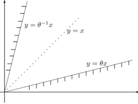
A variation on the theme concerns the same problems when one considers the index setZ^d₊ restricted to asector, which, for the cased= 2, equals

S_θ⁽²⁾={(x, y)∈Z²+:θx≤y≤θ⁻¹x, 0< θ <1}. (3.4) In the limiting case θ= 1, the sector degenerates into a diagonal ray, in which case the sumsSn,n∈S⁽²⁾_θ , are equivalent to the subsequenceSn², more generally, Sn^d, n≥1, of the sequence{Sn, n≥1} whend= 1. In that case it is clear that the usual one-dimensional assumptions are sufficient for the LLN and the LIL.

One may therefore wonder about the proper conditions for the sector—since extra logarithms are needed “at the other end” (asθ→0).

Without going into any details we just mention that it has been shown in Gut (1983) that the law of large numbers as well as the law iterated logarithm hold

(13)

under the same moment conditions as in the cased= 1, and that the limit points in the latter case are the same as in the Hartman–Wintner theorem (Theorem 1.3).

For some additional comments on this we refer to Section 10 toward the end of the paper.

- 6

p pp pp pp pp pp pp pp pp pp pp pp pp pp

y=θ⁻¹x

y=θx y=x

Figure 1: A sector (d= 2)

4. The LLN and LSL for windows

Having defined the general setup we also need the extension of the concept delayed sums or windows to this setting. A window here is an objectTn,n+k. Ford= 2we this is an incremental rectangle

Tn,n+k=Sn1+k1,n2+k2−Sn1+k1,n2−Sn1,n2+k2+Sn1,n2 :

- 6

(n1,n2) (n1+k1,n2)

(n1,n2+k2) (n1+k1,n2+k2 )

q qq qq qq qq qq qq qq qq qq qq qq qq qq qq q

q qq qq qq qq qq qq qq qq qq qq qq qq qq qq q q qq qq qq qq qq qq qq qq qq qq qq qq qq qq q

q qq qq qq qq qq qq qq qq qq qq qq qq qq q q qq qq qq qq qq qq qq qq qq qq qq qq qq qq q

q qq qq qq qq qq qq qq qq qq qq qq qq qq qq q q qq qq qq qq qq qq qq qq qq qq qq qq q

q qq qq qq qq qq qq qq qq qq qq qq q qq qq qq qq qq qq qq qq qq qq q qq qq qq qq qq qq qq qq q q qq qq qq qq qq qq qq q

q qq qq qq qq qq qq q qq qq qq qq qq q qq qq qq q q qq qq q

q qqq q qq qq qq qq qq qq qq qq qq qq qq qq qq q

q qq qq qq qq qq qq qq qq qq qq qq qq q qq qq qq qq qq qq qq qq qq qq qq q qq qq qq qq qq qq qq qq qq q q qq qq qq qq qq qq qq qq q q qq qq qq qq qq qq qq q qq qq qq qq qq qq q qq qq qq qq qq q qq qq qq q q qq qq q q qq

Figure 2: A typical window (d= 2)

(14)

In higher dimensions it is the analogousd-dimensional cube. A strong law for this setting can be found in Thalmaier (2009), Stadtmüller and Thalmaier (2009).

The extension of Theorem 1.8 to random fields runs as follows.

Theorem 4.1. Let 0< α <1, and suppose that {Xk, k∈Z^d₊} are i.i.d. random variables with mean0 and finite variance σ². If

E X^2/α(log⁺|X|)^d⁻¹⁻^1/α<∞, then

lim sup

n→∞

Tn,n+n^α

p2|n|^αlog|n| =σ√

1−α a.s.

Conversely, if

P lim sup

n→∞

|Tn,n+n^α|

p|n|^αlog|n| <∞

>0, thenE X^2/α(log⁺|X|)^d−1−1/α<∞andE X= 0.

Some remarks on the proof will be given in Section 6.

4.1. An LSL for subsequences

The proof of the theorem is in the LIL-style, which, i.a., means that one begins by proving the sufficiency as well as the necessity along a suitable subsequence.

Sticking to this fact one can, with very minor modifications of the proof of Theorem 4.1, prove the followingLSL for subsequences. The inspiration for this result comes from the LIL-analog in Gut (1986).

Theorem 4.2. Let 0 < α < 1, suppose that {Xk,k ∈ Z^d₊} are i.i.d. random variables with mean0 and finite variance σ², and set

Λ ={n∈Z^d₊ :ni =i^β/(1⁻^α), i≥1}. If

E X^2/α(log⁺|X|)^d⁻¹⁻^1/α<∞, then, for β >1,

lim sup

{n→∞n∈Λ^∗}

Tn,n+n^α

p2|n|^αlog|n| =σ

r1−α

β a.s.

Conversely, if

P lim sup

n→∞

{n∈Λ^∗}

|Tn,n+n^α|

p|n|^αlog|n| <∞

>0,

thenE X^2/α(log⁺|X|)^d⁻¹⁻^1/α<∞andE X= 0.

For further details, see Gut and Stadtmüller (2008a), Section 6.

(15)

4.2. Different α:s

During a seminar in Uppsala on the previous material Fredrik Jonsson asked the question: “What happens if theα:s are different?”

In Theorem 4.1 the windows grow at the same rate in each coordinate; the edges of the windows are equal ton^α_k for allk= 1,2, . . . , d. The focus now is to allow for different growth rates in different directions; viz., the edges of the windows will be n^α_k^k,k= 1,2, . . . , d, where, w.l.o.g., we assume that

0< α1≤α2≤ · · · ≤αd<1.

Next, we defineα= (α1, α2, . . . , αd), and set, for ease of notation,

n^α= (n^α₁¹, n^α₂², . . . , n^α_d^d), and |n^α|= Yd k=1

n^α_k^k.

Furthermore, following Stadtmüller and Thalmaier (2009), we letpbe equal to the number ofα:s that are equal to the smallest one.

As for the strong law, the results in Thalmaier (2009), Stadtmüller and Thal- maier (2009), in fact, also cover the case of unequal α:s. For a Marcinkiewicz–

Zygmund analog we refer to Gut and Stadtmüller (2009). For completeness we also mention Gut and Stadtmüller (2010), where some results concerning Cesàro summation are proved.

Here is now the generalization of Theorem 4.1. For a proof and further details we refer to Gut and Stadtmüller (2008b).

Theorem 4.3. Suppose that {Xk, k∈Z^d₊} are i.i.d. random variables with mean 0 and finite varianceσ². If

E|X|^2/α¹(log⁺|X|)^p⁻¹⁻^1/α¹ <∞, then

lim sup

n→∞

Tn,n+n^α

p2|n^α|log|n| =σ√

1−α1 a.s.

Conversely, if

P lim sup

n→∞

|Tn,n+n^α|

p|n^α|log|n| <∞

>0, thenE|X|^2/α¹(log⁺|X|)^p⁻¹⁻^1/α¹<∞ andE X= 0.

Remark 4.4. If α1 = α2 = · · · = αd = α, thenp = dand |n^α| = |n|^α, and the theorem reduces to Gut and Stadtmüller (2008a), Theorem 2.1 = Theorem 4.1 above.

Remark 4.5. For a result for subsequences analogous to Theorem 4.2; see Gut and Stadtmüller (2008b), Section 6.

(16)

We observe that the moment condition as well as the extreme limit points depend on thesmallest αand its multiplicity. Heuristically this can be explained as follows. The longer the stretch of the window along a specific axis, the more cancellation may occur in that direction. Equivalently, the shorter the stretch, the wilder the fluctuations. This means that in order to “tame” the fluctuations it is (only) necessary to put conditions on the shortest edge(s).

4.3. Different α:s, log, and log log

One can exaggerate the mixtures even further, namely, by combining edges that expand at different α-rates with edges that expand with different almost linear rates. Some results in this direction concerning the LLN can be found in Gut and Stadtmüller (2011b).

The paper Gut and Stadtmüller (2011a) is devoted to the LSL. First a result from that paper that extends Gut et al. (2010) to random fields for (iterated) logarithmic expansions and mixtures of them. For simplicity and illustrative purposes we stick to the cased= 2.

Theorem 4.6. Let {Xi,j, i, j≥1}be i.i.d. random variables.

(i)If

E X² (log⁺|X|)³

log⁺log⁺|X| <∞ and E X = 0, E X²=σ², then

lim sup

m,n→∞

T_(m,n)_,(m+m/_log_m,n+n/_log_n) q4mn^{log log}_log^{m+log log}_mlog_n ⁿ

=σ a.s.

Conversely, if P

lim sup

n→∞

|T(m,n),(m+m/logm,n+n/logn)| q

mn^{log log}_log^{m+log log}_m_log_n ⁿ

<∞

>0,

thenE X^{2 (log}_log+⁺log^|^X⁺^||⁾X³|<∞ andE X= 0. (ii)If

E X²log⁺|X|log⁺log⁺|X|<∞ and E X= 0, E X²=σ², then

lim sup

m,n→∞

T(m,n),(m+m/log logm,n+n/log logn)

q2mn^{log log}_{log log}^{m+log log}_{mlog log}_nⁿ

=σ a.s.

Conversely, if P

lim sup

n→∞

|T(m,n),(m+m/log logm,n+n/log logn)| q

mn^{log log}_{log log}^{m+log log}_m_{log log}_nⁿ

<∞

>0,

(17)

thenE X²log⁺|X|log⁺log⁺|X|<∞andE X= 0.

(iii)If

E X²(log⁺|X|)²<∞ and E X= 0, E X²=σ², then

lim sup

m,n→∞

T(m,n),(m+m/logm,n+n/log logn)

q4mn^{log log}_log_m^{m+log log}_{log log}_nⁿ

=σ a.s.

Conversely, if P

lim sup

n→∞

|T(m,n),(m+m/logm,n+n/log logn)| q4mn^{log log}_log_m^{m+log log}_{log log}_nⁿ

<∞

>0,

thenE X²(log⁺|X|)²<∞andE X = 0.

We conclude with an example where a logarithmic expansion is mixed with a power.

Theorem 4.7. Let 0< α <1, and let {Xi,j, i, j ≥1} be i.i.d. random variables.

If

E X^2/α(log⁺|X|)⁻^1/α<∞ and E X= 0, E X²=σ², then

lim sup

m,n→∞

T(m,n),(m+m^α, n+n/logn)

q

2m^αn⁽¹⁻^{α) log(mn)}_log_n

=σ a.s.

Conversely, if P

lim sup

m,n→∞

|T(m,n),(m+m^α, n+n/logn)| q

m^αn^log(mn)_log_n

<∞

>0,

thenE X^2/α(log⁺|X|)⁻^1/α<∞ andE X= 0.

5. Preliminaries

Proposition 5.1. Let r >0 and letX be a non-negative random variable. Then

E X^r<∞ ⇐⇒

X∞ n=1

n^r−1P(X ≥n)<∞,

More precisely, X∞ n=1

n^r−1P(X ≥n)≤E X^r≤1 + X∞ n=1

n^r−1P(X ≥n).

(18)

As an example, consider the case r = 1, and suppose that X1, X2, . . . is an i.i.d. sequence. It then follows from the proposition that, for anyε >0,

P(|Xn|> nεi.o.) = 0 ⇐⇒

X∞ n=1

P(|Xn|> nε)<∞ ⇐⇒ E|X|<∞.

Suppose instead that we are facing an i.i.d. random field{Xn,n∈Z^d₊}. What is then the relevant moment condition that ensures that

X

n

P(|Xn|>|n|)<∞? or, equivalently, that X

n

P(|X|>|n|)<∞? (5.1) In order to answer this question it turns out that we need the quantities

d(j) = Card{k:|k|=j} and M(j) = Card{k:|k| ≤j}, which describe the “size” of the index set, and their asymptotics

M(j)

j(logj)^d−1 → 1

(d−1)! and d(j) =o(j^δ)for anyδ >0 as j→ ∞; (5.2) cf. Hardy and Wright (1954), Chapter XVIII and Titchmarsh (1951), relation (12.1.1) (for the cased= 2). The quantityd(j)itself has no pleasant asymptotics;

lim infj→∞d(j) =d, and lim sup_j_→∞d(j) = +∞.

Now, exploiting the fact that all terms in expressions such as the second sum in (5.1) with equisized indices are equal, we conclude that

X

n

P(|X|>|n|) = X∞ j=1

X

|n|=j

d(j)P(|X|> j), (5.3) which, via partial summation yields the first half of following lemma. The second half follows via a change of variable.

Lemma 5.2. Let r >0, and suppose thatX is a random variables. Then X

n

P(|X|>|n|)<∞ ⇐⇒ E M(|X|)<∞ ⇐⇒ E|X|(log⁺|X|)^d⁻¹<∞, X

n

|n|^r⁻¹P(|X|>|n|)<∞ ⇐⇒ E M(|X|^r)<∞ ⇐⇒ E|X|^r(log⁺|X|)^d⁻¹<∞.

Reviewing the steps leading to the lemma one finds that if, instead, we consider the sector (recall (3.4)) one finds that

X

n∈Sθ^d

P(|X|>|n|)<∞ ⇐⇒ E M(|X|)<∞ ⇐⇒ E|X|<∞. (5.4) Remark 5.3. Note that the first equivalence is the same as in Lemma 5.2, and that the second one is a consequence of the “size” of the index set.

(19)

For results such as Theorem 4.3, as well as for some of the results in Section 8 below, we shall need the more general index sets

Mα(j) = Card{k:|k^α| ≤j^α¹}= Card{k: Yd ν=1

k_ν^α^ν^/α¹ ≤j}. (5.5) Generalizing Lemma 3 in Stadtmüller and Thalmaier (2009) in a straight forward manner yields the following analog of (5.2):

Mα(j)∼cαj(logj)^p−1 as j→ ∞ (5.6) wherecα>0, which, in turn, via partial summation, tells us that

X

n

P(|X|>|n^α|) X∞ j=1

(logj)^p−1P(|X|> j^α¹).

Using a slight modification of this, together with the fact that the inverse of the functiony =x^α(logx)^κ behaves asymptotically likex=y^1/α(logy)⁻^(κ/α), yields the next tool (Gut and Stadtmüller (2008a), Lemma 3.2, Gut and Stadtmüller (2008b), Lemma 3.1).

Lemma 5.4. Let κ∈Rand suppose that X is a random variable. Then, X

n

P |X|>|n^α|(log|n|)^κ

<∞ ⇐⇒ E|X|^1/α¹(log⁺|X|)^{p−1−κ/α}¹ <∞.

In particular, ifα1=α2=· · ·=αd=κ= 1/2, then X

n

P |X|>p

|n|log|n|

<∞ ⇐⇒ E X²(log⁺|X|)^d⁻²<∞.

For illustrative reasons we also quote Gut and Stadtmüller (2008a), Lemma 3.3, as an example of the kind of technical aid that is required at times.

Lemma 5.5. Let κ≥1,θ >0, andη∈R.

X∞ i=2

X

{n:|n|=i^κ(logi)^η}

1

|n|^θ = X∞ i=2

d(i^κ(logi)^η) i^κθ(logi)^ηθ





<∞, when θ > ¹_κ,

=∞, when θ < ¹_κ.

6. Sketch of the proofs of Theorems 4.1 and 4.3

In this section we give som hints on the proofs of Theorems 4.1 and 4.3, in the sense that we shall point to differences and modifications compared to the proof of Theorem 2.2 in Section 2.2.

(20)

6.1. On the proof of Theorem 4.1

This time truncation is at bn=b_|n|= σδ

ε p|n|^α

log|n| and cn=δp

|n|^αlog|n|, for some (arbitrarily) smallδ >0.

The first step differs slightly from the analog in the proof of Theorem 2.2, in that we now start by dispensing of the full double- and triple primed sequences (recall Remark 2.8).

As for the double primed contribution we argue that in order for the|T_n,n+n⁰⁰⁰ ^α|:s to surpass the level ηp

|n^α|log|n| infinitely often, for some η > 0 small, it is necessary that infinitely many of the X⁰⁰⁰:s are nonzero, and the latter event has probability zero by the first Borel–Cantelli lemma, since

X

n

P(|Xn|> ηp

|n|^αlog|n|) =X

n

P(|X|> ηp

|n|^αlog|n|)<∞,

where the finiteness is a consequence of the moment assumption and the second half of Lemma 5.4.

Taking care of T_n,n+n⁰⁰ ^α is a bit easier this time, the argument being that in order for |T_n,n+n⁰⁰ ^α|to surpass the levelηp

|n|^αlog|n|it is necessary that at least N ≥η/δ of the X⁰⁰:s are nonzero, which, by stretching the truncation bounds to the extremes, some elementary combinatorics, and the moment assumption implies that

P(|T_n,n+n⁰⁰ ^α|> ηp

|n|^αlog|n|)

≤ |n|^α

N

P bn<|X| ≤δp

(|n|+|n|^α) log(|n|+|n|^α)^N

≤C(log|n|)^N^((3/α)+1⁻^d)

|n|^N(1−α) , and, hence, that

X

n

P(|T_n,n+n/L(n)⁰⁰ |> ηp

|n|^αlog|n|)<∞ for all η > δ 1−α,

wheneverN(1−α)>1 (andN δ≥η), after which another application of the first Borel–Cantelli lemma concludes that part of the proof.

As forT_n,n+n⁰ ^α, the exponential bounds do the job as before;

P T_n,n+n⁰ ^α> εp

2|n|^αlog|n|







≤exp

−2ε²(1−δ)²

2σ² log|n|(1−δ) ,

≥exp

−2ε²(1 +δ)²

2σ²(1−δ) log|n|(1 +γ) .

(21)

Putting things together proves the theorem for suitably selected subsequences, and thus, in particular also the lower bound for the full field (remember Step 12 in the skeleton list).

It thus remains to verify the upper bound for the entire field.

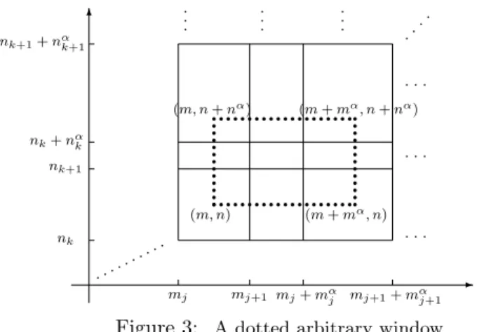
Now, for the LIL and LSL one investigates the gaps between subsequence points with the aid of the Lévy inequalities, as we have seen in the proof of Theorem 2.2, Step 6. When d≥2, however, there are no gaps in the usual sense and one must argue somewhat differently.

Let us have a quick look at the situation when d = 2. First we must show that the selected subsequence (which we have not explicitly presented) is such that the subset of windows overlap, viz., that they cover all ofZ²₊. Next, we select an arbitrary window

T((m,n),(m+m^α,n+n^α))

and note that it is always contained in the union of (at most) four of the earlier selected ones:

- 6

p p p pp p p pp p

p pp p

p p p p p p p p p ppp

ppp

qqqq qqqq qqqq

q q q q q q q q q q q q q q q q q q q q q q q q q q q q q q q q q q q q q q q q

qqqq qqqq qqqq q

(m, n) (m+m^α, n) (m, n+n^α) (m+m^α, n+n^α)

m_j m_j+1 mj+m^α_j mj+1+m^α_j+1 n_k

nk+1

nk+n^α_k n_k+1+n^α_k+1

Figure 3: A dotted arbitrary window

One, finally, shows that the discrepancy between the arbitrary window and the selected ones is asymptotically negligible. This is a technical matter which we omit. Except for mentioning that one has to distinguish between the cases when the arbitrary window is located in “the center” of the index set or “close” to one of the coordinate axes (for a similar discussion cf. also Gut (1980), Section 4).

6.2. On the proof of Theorem 4.3

This proof runs along the same lines as the previous one with some additional technical complications, due to the non-equalness of theα:s. In order to illustrate this, consider the triple-primed windows.

Truncation now is at bn=b_|n|= σδ

ε

p|n^α|

log|n| and cn=δp

|n^α|log|n|,

(22)

forδ >0small; note|n^α|instead of|n|^α.

The argument forT_n,n+n⁰⁰⁰ ^α:s is verbatim as before, and leads to the sum X

n

P(|Xn|> ηp

|n^α|log|n|) =X

n

P(|X|> ηp

|n^α|log|n|)<∞,

where the finiteness is a consequence of the moment assumption, which this time is a consequence of the first half of Lemma 5.4.

The remaining part of the proof amounts to analogous changes.

7. The Hsu–Robbins–Erdős–Spitzer–Baum–Katz theorem

One aspect of the seminal paper Hsu and Robbins (1947) is that it started an area of research related to convergence rates in the law of large numbers, which, in turn, culminated in the now classical paper Baum and Katz (1965), in which the equivalence of (7.1), (7.2), and (7.4) below was demonstrated. Namely, in Hsu and Robbins (1947) the authors introduced the concept of complete convergence, and proved that the sequence of arithmetic means of i.i.d. random variables converges completely to the expected value of the variables provided their variance is finite.

The necessity was proved by Erdős (1949, 1950).

Theorem 7.1. Let r > 0, α > 1/2, and αr ≥1. Suppose that X1, X2, . . . are i.i.d. random variables with partial sumsSn =Pn

k=1Xk,n≥1. If

E|X|^r<∞ and, if r≥1, E X= 0, (7.1) then

X∞ n=1

n^αr⁻²P(|Sn|> n^αε)<∞ for all ε >0; (7.2) X∞

n=1

n^αr⁻²P( max

1≤k≤n|Sk|> n^αε)<∞ for all ε >0. (7.3) If αr >1we also have

X∞ n=1

n^αr⁻²P(sup

k≥n|Sk/k^α|> ε)<∞ for all ε >0. (7.4) Conversely, if one of the sums is finite for all ε > 0, then so are the others (for appropriate values ofrand α),E|X|^r<∞and, if r≥1,E X= 0.

The Hsu–Robbins–Erdős part corresponds to the equivalence of (7.1) and (7.2) for the caser= 2andp= 1. Spitzer (1956) verified the same for the caser=p= 1, and Katz (1963), followed by Baum and Katz (1965) took care of the equivalence