Control of epidemic propagation on networks by using a mean-field model
Dedicated to Professor László Hatvani on the occasion of his 75th birthday
Ágnes Bodó
1, 2and Péter L. Simon
B1, 21Institute of Mathematics, Eötvös Loránd University, 1/C Pázmány P. s., Budapest, H–1117, Hungary
2Numerical Analysis and Large Networks Research Group, Hungarian Academy of Sciences, Hungary
Received 2 January 2018, appeared 26 June 2018 Communicated by Gergely Röst
Abstract. Epidemic propagation is controlled conventionally by vaccination or by quar- antine. These methods have been widely applied for different compartmental ODE models of epidemic propagation. When epidemic spread is considered on a network, then it is natural to control the propagation process by changing the network struc- ture. Namely,SI links, connecting a susceptible individual to an infected one, can be deleted. This would lead to a disconnected network, which is not realistic, hence new SSlinks can be created in order to keep the network well connected. Thus it seems to be promising to drive the process to a target with no infection and a prescribed average degree by deletingSI links and creatingSSlinks in an appropriate way. It was shown previously that this can be done for the pairwise ODE approximation ofSISepidemic propagation. In this paper this is extended to the original stochastic process by using the control signals computed from the ODE approximation.
Keywords: SIS epidemic, pairwise model, adaptive network, nonlinear model predic- tive control, individual-based simulation.
2010 Mathematics Subject Classification: 34H20, 05C82, 65C40, 92D30.
1 Introduction
Deriving mathematical models of epidemic propagation was primarily and originally moti- vated by the need of controlling the spread of a disease. This demand has led to several modeling approaches starting from compartmental models to network-based models with different complexity, such as mean-field, pairwise, compact pairwise, degree based or indi- vidual based models [1,10,13,15]. All of these models are systems of non-linear differential equations, placing the problem of epidemic control into control theory [8,19], a well-developed
BCorresponding author.
Emails: bodoagi@cs.elte.hu (Á. Bodó), simonp@cs.elte.hu (P. L. Simon)
field of mathematics motivated mainly by engineering problems. Similarly to other questions, the control of epidemics can be formalised in the language of optimal control. The target is to drive the number of infected individuals to zero (or at least decreasing it as much as possible).
This could be simply achieved by separating all the individuals from each other or vaccinating or treating all of them. This intervention obviously generates a cost that can be quantified by a cost function, the value of which is minimised.
Most models use vaccination or treatment as control measures, hence the cost function incorporates the cost of the vaccine or medical treatment [3,9,12]. Since the literature of epidemic control is extremely rich, we mention here briefly only those results that are signifi- cantly relevant from the point of view of our study. The optimal time dependent vaccination was investigated in a susceptible-infected-recovered (SIR) model under minimising a cost function that measures the cumulative amount of infected and vaccinated people [16]. Clancy and Piunovsky [3] computed optimal control based on isolation in a variant of the classical SIR model with nonlinear infection rate function. Hansen and Day [9] considered optimal control in the presence of limited resources using isolation, vaccination and mixed control strategies for theSIR dynamics. The application of optimal control theory to SIR propaga- tion on networks in a real world situation is presented in [17]. The effect of vaccination in an SIRS model on heterogeneous networks is studied in [2]. These models are typically based on compartments of individuals in different states of the disease, in different age or place of working and living. Quarantine and contact tracing offer another control measure that uses information about the relation among the individuals in a certain sense [11,14].
An alternative is to incorporate the contact structure of the individuals and use the dele- tion or creation of links between them as control measure [18]. This has been carried out for the pairwiseSIS(susceptible–infected–susceptible) model in [18], where nonlinear model predictive control was applied to drive the number of infected nodes in the network to zero while keeping the network well connected. In that paper, theSI edges (connecting a suscep- tible and an infected node) are cut to eradicate disease andSSedges are created to maintain a given average degree in the network.
In this paper, we make a further step towards network-based epidemic control. The differ- ential equation models of epidemic propagation on networks are approximations of the real process since all of them contain closure relations. Thus it is natural to ask how the original process can be controlled. The full stochastic model has an enormously large state space (for SISepidemic on a network with Nnodes, the state space has 2N elements), hence individual based stochastic simulation is used to follow the process. Our goal in this paper is to con- trol the stochastic simulation itself. We will study to what extent the control predicted by a network-based reduced ODE model results in good control of the full stochastic model. Stud- ies in this direction already exist, and the first signs are positive. Namely, control computed from mean-field models seem to translate well, at least for some cases, for the control of the stochastic simulation counterpart [4,20]. Our approach is motivated also by the fact that the cost of computing control from ODEs is much smaller than that of working out control from stochastic models. The main idea of our approach can be summarised briefly as follows. The process is controlled by cutting SI and creating SS edges in the stochastic simulation. The number of edges to be created or to be deleted is determined from the pairwise ODE model by updating its initial condition at the time instantsk∆t, with an appropriately chosen time step∆t, by using the values obtained from the stochastic simulation.
The results of our study are the following. On the one hand, we found that computing the values of the control parameters from the ODE approximation can be used to control
the stochastic simulation. On the other hand, the success of the control strongly depends on the epidemic parameters, the infection and recovery rate, and on the control parameters, the length of the time horizon, the time step ∆t, of updating the control parameter values, and the parameters of the optimisation process in the model predictive control. We will show numerical evidence that the stochastic simulation can be controlled by using the control signals obtained from the ODE approximation, if the time step∆tis small enough. The effect of the control bounds on the controllability will also be studied in detail.
The paper is structured as follows. In Section 2 our stochastic model for SIS epidemic propagation on an adaptive network and its pairwise ODE approximation are introduced.
The detailed description of the control method is given in Section 3 both for the stochastic simulation and for the pairwise ODE. The results about the controllability of the simulation are presented in Section4.
2 Model formulation
In this section the mathematical model ofSIS epidemic propagation on an adaptive network with link-type dependent link activation and deletion is presented. To describe the model con- sider an undirected simple graph with Nnodes, where each node can be either susceptible (S) or infected (I). A susceptible node can become infected when contacted with an infected one, and an infected one can recover and become susceptible again. In order to avoid infection, it is reasonable to assume that susceptible nodes break their links to infected ones and reconnect to a randomly chosen susceptible node, moreover susceptible nodes may cancel their links to other susceptible ones in order to avoid a possible infection if the neighbour becomes infected.
Hence in our model it is possible to create new links and to delete existing connections leading to changes in the network structure.
In the standard adaptiveSIS model, infection, recovery, link activation and link deletion are governed by independent Poisson processes. A susceptible node becomes infected at rate kτ, where k is the number of its infected neighbours and τ > 0 is a given constant, called infection rate. Each infected node recovers at rate γ, whereγ > 0 is called the recovery rate.
A non-existing link between two nodes of type A ∈ {S,I} and B ∈ {S,I} is activated at rate αAB. Similarly, an existing link between a node of type A ∈ {S,I}and a node of type B ∈ {S,I} is terminated at rate ωAB. The graph is assumed to be undirected, therefore we assume that αSI=αIS andωSI =ωIS.
The mathematical model of the process is a system of ordinary differential equations, called master equations that consists of differential equations for the time dependent proba- bilities of each state. The state space of the adaptive SISmodel on a networks with Nnodes contains
2N
|{z}
nodes
·2N(N2−1)
| {z }
edges
elements, because every node can be either susceptible or infected and every link can be either existing or non-existing. Therefore, even writing down the differential equations is not feasible for large N. To demonstrate the complexity of the problem let us take a look at the case N = 2. LetXAB denote the probability of the state, in which the first node is of type A and is connected to the second one, which is of typeB. Similarly, the probability of the state where there is no link between the nodes is denoted by XAB. The master equations take the
following form:
X˙SS=γ XSI+XIS
+αSSXSS−ωSSXSS, X˙SS=γ(XSI+XIS) +ωSSXSS−αSSXSS, X˙SI =γXI I+αSIXSI−(γ+τ+ωSI)XSI, X˙SI =γXI I+ωSIXSI−(γ+αSI)XSI, X˙IS =γXI I+αSIXIS−(γ+τ+ωSI)XIS, X˙IS =γXI I+ωSIXIS−(γ+αSI)XIS,
X˙I I =τ XSI+XIS
+αI IXI I−(2γ+ωI I)XI I, X˙I I =ωI IXI I−(2γ+αI I)XI I,
where dot denotes differentiation with respect to time.
In order to overcome this difficulty, approximating non-linear differential equations have been derived for coarse-grained variables. This can be done at the individual level or at the population level. One of the latter is presented in the next section.
2.1 Pairwise model
A widely used population level approximation is the so-called pairwise model. This is for- mulated in terms of the number of nodes and edges in different states, hence it is suitable for incorporating the control action as creating and deleting certain types of links. The pairwise model for the expected values of the number of nodes and links takes the form (see Chapter 8 in [15])
[I˙] =τ[SI]−γ[I], (2.1)
[SI˙ ] =−(τ+γ)[SI] +τ([SSI]−[ISI]) +γ[I I] +αSI([S][I]−[SI])−ωSI[SI], (2.2) [SS˙ ] =2γ[SI]−2τ[SSI] +αSS([S]([S]−1)−[SS])−ωSS[SS], (2.3) [I I˙ ] =−2γ[I I] +2τ([ISI] + [SI]) +αI I([I]([I]−1)−[I I])−ωI I[I I], (2.4) where [I](t) and [S](t) are the expected values of the number of infected and susceptible nodes at timet, ([S](t) + [I](t) =Nholds for allt),[SI](t),[I I](t),[SS](t)denote the expected number ofSI, I I andSSedges and [SSI](t),[ISI](t)denote the expected number ofSSI, ISI triples at timet. System (2.1)–(2.4) is not self-contained in this form, since there are no equa- tions for the number of triples. Instead of deriving differential equations for those variables, an approximating algebraic relation is used typically to express the number of triples in terms of the pairs and singles. The most frequently used and widely accepted approximation is the following [10]:
[SSI] = n−1 n
[SS][SI]
[S] = n−1 n
[SS][SI] N−[I], [ISI] = n−1
n
[SI][SI]
[S] = n−1 n
[SI][SI] N−[I],
where Nis the size of the population andn =n(t)is the actual mean degree of the network, i.e.
n(t) = [SS] +2[SI] + [I I]
N .
2.2 Network-based stochastic model
The stochastic simulation is based on the Gillespie algorithm ([6], [7]), which we have imple- mented in MATLAB. Let[0,T]be the time interval of the simulation. Moreover, letG = (V,E) be the initial graph, where V andE represent the nodes and the edges of the graph, respec- tively. A node v ∈ V can be susceptible or infected and an edgee ∈ E can be of typeSI, SS or I I. Let us assume that the parameters N= |V |,τ, γ,αSS,αSI, αI I, ωSS,ωSI and ωI I are all given.
The simulation is based on an accurate book keeping of all possible events, i.e. a node may become infected or susceptible, or an edge is created or removed. The most important step of the algorithm is to compute the rates of all possible events. These rates can be represented with a vectorr of size
N
|{z}
nodes
+ N(N−1) 2
| {z }
edges
,
where the firstNelements correspond to the events related to the nodes (infection and recov- ery) and the remaining N(N−1)/2 elements of r refer to the edges (creation and deletion).
For instance, in case a node v is infected, i.e. it may recover, the rate corresponding to this node is γ. In case v is susceptible with k infected neighbours, its corresponding rate is kτ.
An existing linkAB ∈ {SS,SI,I I}can be removed, therefore the corresponding rate isωAB. Furthermore a non-existing linkAB ∈ {SS,SI,I I}can be created, therefore the rate belonging to it isαAB.
Let R denote the sum of the rates, i.e. R = ∑ir(i). The next step is to specify the timet of the next event. To determine this we choose a random number from an exponential dis- tribution with parameter R. Next we determine which event will be performed. The event is chosen randomly but proportionally to its rate and may correspond to either a node or an edge. Once the event is chosen we update the graph G, i.e. the states of the nodes and the edges. After that using the new graph G the rates of the events are calculated, then a new time stept is determined and the next event is chosen randomly again.
Given that all existing and non-existing links need to be accounted for, the algorithm which includes the storage, update and referencing back and forth between rates and events becomes more complex.
3 Dynamic control of the adaptive SIS model
Now we turn to the main goal of the paper, to investigate the controllability of the adaptive SIS epidemic on a network by creating and deleting edges. Our aim is to eradicate the epidemic and keep the network well connected as well, i.e. to lead the system to the state when the expected number of infected nodes is [I](T) = I∗ and the average degree is n(T) = n∗ for some finite T>0 and target valuesI∗ =0 andn∗ =n(0).
In order to achieve our goal we change the rates of creation and deletion ofSSlinks and deletion ofSIlinks from time to time. This process models that healthy people terminate their connections to infected ones and try to find connections to other healthy individuals in order not to be disconnected socially. Thus in our control process we have
αSI =αI I =ωI I =0, ωSI =u1 (3.1) and
αSS =u2, ifu2>0, ωSS=−u2if u2<0, (3.2)
where u1 and u2 are our control parameters. Since we use time dependent control, u1 and u2 will be piecewise constant functions. We fix a step size∆t > 0 determining how often we intervene and change the values of the control parameters. That is the control functions u1 andu2 will be constant in each time interval[(k−1)∆t,k∆t), fork =1, 2, . . . ,KwithK∆t =T.
Furthermore we assume that the control parameters are bounded, namely there exist pos- itive numbersM1and M2, such that
0≤u1(t)≤ M1, |u2(t)| ≤ M2 for allt∈ [0,T]. (3.3) We define the controllability of our system as follows.
Definition 3.1. The system isε-controllable to the target values I∗ =0 andn∗ =n(0)with pa- rametersT,∆t, M1, M2, if there are piecewise constant functionsu1,u2: [0,T]7→R, such that (3.3) holds andu1 andu2 are constants in the intervals [(k−1)∆t,k∆t)for all k = 1, 2, . . . ,K, furthermore
|[I](T)−I∗| ≤ε, |n(T)−n∗| ≤ε.
In practice, the caseε=0, i.e. perfect controllability is not expected.
In the next subsections we show how the control functions u1 and u2 are determined for the pairwise model and for the stochastic simulation.
3.1 Time dependent control of the pairwise model
Using the parameter values given in (3.1)–(3.2), system (2.1)–(2.4) takes the following form:
[I˙] =τ[SI]−γ[I], (3.4)
[SI˙ ] =−(τ+γ)[SI] +τ([SSI]−[ISI]) +γ[I I]−u1[SI], (3.5) [SS˙ ] =2γ[SI]−2τ[SSI] +max{u2, 0}([S]([S]−1)−[SS]) +min{u2, 0}[SS], (3.6) [I I˙ ] =−2γ[I I] +2τ([ISI] + [SI]). (3.7) Our aim now is to determine the values of the piecewise constant functionsu1andu2in such a way that system (3.4)–(3.7) becomesε-controllable. This has already been carried out in [18]
by using nonlinear predictive control. Here we only briefly summarize the main steps of the method because these control signals will be used to control the stochastic simulation in the next subsection.
The Nonlinear Model Predictive Control (NMPC), which is a variant of Model Predictive Control (MPC), is an optimization based method for the feedback control of nonlinear systems.
It is widely applied to stabilization and tracking problems, see [8].
First, we discretize system (3.4)–(3.7) in order to apply the NMPC algorithm. In order to make the equations simpler use the following vectorial notations:
X= ([I],[SI],[SS],[I I]), U= (u1,u2).
Let us denote the output variables, i.e. the number of infected individuals and the mean degree, by Y = ([I],n). We use Xi and Yi for the i-th coordinate of X and Y respectively, and x(k) = X(k∆t), y(k) = Y(k∆t), u(k) = U(k∆t). Let us denote the solution operator of system (3.4)–(3.7) byφ, that is the solution starting from the initial conditionX(0)is given by X(t) =φ(t,X(0),U(t)). Now, the control is constant in a time interval of length∆t, hence we will use the discretized solution function
F(x,u) =φ(∆t,x,u), (3.8)
wherex∈ R4andu∈R2are given vectors. Furthermore, we introduce the discretized output function as
H(x) = (x1,(x3+2x2+x4)/N), (3.9) the first coordinate of which is[I]and its second coordinate is the average degree.
Following [18], we compute the control actionuat timek∆tin the following way. First, we set a prediction horizon of lengthPsteps and denote byui(k+j)fori=1, 2, j=0, 1, . . . ,P−1 an arbitrary admissible future control action chosen at time k∆t. Given this control sequence, the solution at the end points of the time steps starting from x(k) =X(k∆t)is given as
x(k+1) =F(x(k),u(k)), x(k+2) =F(x(k+1),u(k+1)), . . . i.e. in general
x(k+j) =F(x(k+j−1),u(k+j−1)), for j=1, 2, . . .P.
The output variables are simply given as
y(k+j) =H(x(k+j)), for j=1, 2, . . .P.
Now comes the most important step, to compute the sequence of control valuesu(k),u(k+1), . . .,u(k+P−1)in such a way that the output values y(k+1), y(k+2), . . ., y(k+P) get as close to the target value(I∗,n∗)as possible. This can be achieved by minimising the objective functionalJ :R2P →Rgiven as
J (u(k), . . . ,u(k+P−1))
=
∑
P j=1λ1(y1(k+j)−I∗)2 +λ3(∆u1(k+j))2+λ2(y2(k+j)−n∗)2+λ4(∆u2(k+j))2, where λ1,λ2,λ3,λ4 are parameters (damping parameters) and ∆ui(k+ j) = ui(k+ j)− ui(k+j−1)is the change of control value from thek-th time step to the next one. We solve the above nonlinear optimization problem using the so-called lsqnonlin optimization routine in MATLAB, yielding values for the control values u(k),u(k+1), . . .,u(k+P−1). Then the control signal u(k)is used in the time interval [k∆t,(k+1)∆t)and the whole computation is repeated at time(k+1)∆tto obtain the control signal in the interval[(k+1)∆t,(k+2)∆t)and so on until the end of the time interval, T, is reached.
It was shown in [18] that choosing the control parameters appropriately, system (3.4)–(3.7) is ε-controllable for small values of ε, i.e. Y(T) will be sufficiently close to the target value (I∗,n∗). In the next subsection, this result is applied to control the stochastic simulation.
3.2 Control of the network-based stochastic model
Now our aim is to control the network-based stochastic model. The question is how to choose the control parameters in order to control the simulation. The idea for controlling the pairwise model was to determine the output for an arbitrary admissible control sequence and then minimising the objective function to get the best control signal. In the case of the stochastic simulation, the difficulty is in computing the output for several different control sequences.
Hence the idea is to use the control values obtained for the pairwise model in order to control the simulation.
Let us assume that the model parameters N, τ, γ, I(0), n(0) and the control parameters P, λ1, λ2, λ3,λ4, T and ∆t are given. We determine the control values u1 andu2 in the time intervals[(k−1)∆t,k∆t), fork =1, 2, . . . ,Kwith K∆t= Tin two different ways.
(A) One way of doing so is simply determine u(k) for k = 1, 2, . . . ,K from the pairwise model by using the above described NMPC algorithm and starting from the initial state.
These control values can then be used in the stochastic simulation in the time intervals [(k−1)∆t,k∆t). This will be presented in Section 4.1. However, as we will see in the next section, these control values will not work well since the pairwise model is not an accurate approximation of the stochastic simulation.
(B) The second way of determining the control signals, presented in Section 4.2, is the following. Compute u(1) from the pairwise model by using the NMPC algorithm described above and starting from the initial state. Then applyu(1) in the time interval [0,∆t) for the stochastic simulation and denote by x(1) the state to which the simulation arrives at time
∆t. In the next stage compute u(2)from the pairwise model by using the NMPC algorithm described above and starting from the statex(1). Then applyu(2)in the time interval[∆t, 2∆t) for the stochastic simulation and denote by x(2)the state to which the simulation arrives at time 2∆t. These steps are repeated until the end of the time interval, T, is reached. Thus, in each time step, the state of the system is determined by using the stochastic simulation and the control values are determined from the pairwise ODE model.
4 Simulation results
In this section we present numerical results for controlling the stochastic simulation, for which we showed two methods in Section3.2. In the first subsection we show that the first method is not able to lead the system to the target. Then, in the second subsection, successful control results, obtained by the second method, are presented.
4.1 Control of the stochastic model by using method (A)
Extensive numerical simulations were carried out for the pairwise model in [18]. These showed that for fixed value of τ and M2 there is a critical value of M1, such that the con- trol is effective whenM1is larger than this threshold. First, we chose a value ofτ, M1andM2, for which the control of the pairwise model is effective and determined the control values for each time step. Then we applied these control signals to the stochastic simulation. The result is presented in Figure4.1 showing that the solution of the pairwise model reaches the target values (I∗ = 0 and n∗ = 10), while prevalence obtained from the simulation does not drop to zero and the average degree is well above the target. This means that the control signal obtained from the pairwise model is not effective for the stochastic simulation.
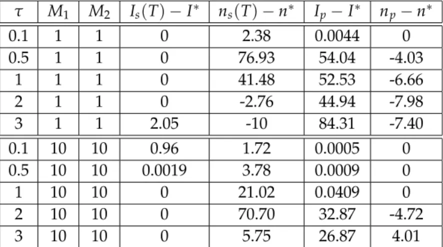
We repeated this experiment with several values of τ, M1 andM2. For each triple, we de- termined the control signals from the pairwise model and then applied these in the stochastic simulation. The difference of the actual and target values of the prevalence and average de- gree at time T are shown in Table 4.1. One can see that the pairwise model is controllable when τ is not too large, while the stochastic simulation does not reach the target even for small values ofτ.
This shows that the first method does not yield effective control for the stochastic simula- tion. This has led us to the application of the second method.
t
0 2 4 6 8 10
I(t), n(t)
0 2 4 6 8 10 12 14
Is ns Ip np
Figure 4.1: Time evolution of the prevalence (red) and average degree (blue) in the pairwise model (dashed) and in the stochastic simulation (continuous curves) for N= 100,τ= 2,γ =1, I(0) = 10, I∗ =0, n(0) =n∗ = 10,∆t =0.1, λ1=λ2 =104,λ3 =λ4=1, M1= M2=100.
τ M1 M2 Is(T)−I∗ ns(T)−n∗ Ip−I∗ np−n∗
0.1 1 1 0 2.38 0.0044 0
0.5 1 1 0 76.93 54.04 -4.03
1 1 1 0 41.48 52.53 -6.66
2 1 1 0 -2.76 44.94 -7.98
3 1 1 2.05 -10 84.31 -7.40
0.1 10 10 0.96 1.72 0.0005 0
0.5 10 10 0.0019 3.78 0.0009 0
1 10 10 0 21.02 0.0409 0
2 10 10 0 70.70 32.87 -4.72
3 10 10 0 5.75 26.87 4.01
Table 4.1: Difference between the prevalence and average degree and their target for different values of τ, M1 and M2 for N = 100, γ = 1, I(0) = 10, I∗ = 0, n(0) =n∗ =10, ∆t =0.1,λ1 =λ2 =104,λ3=λ4=1.
4.2 Control of the stochastic model by using method (B)
Now we present successful control results obtained by applying the second method. We recall that in this case the control signal in the time interval[(k−1)∆t,k∆t)is computed from the pairwise model but the initial condition at time (k−1)∆t is taken from the stochastic simulation.
A successful control process is shown in Figure 4.2, where the time dependence of the prevalence, average degree and the control signals are shown. One can see that the link deletion rate,u1is at the maximum value,M1in the first part of the process. The creation and deletion of SSlinks,u2, shows an interesting time dependence. First, it is negative, that isSS links are deleted (in order to prevent strong propagation), then SSlinks are created in order
to achieve the target value of the average degree. We note that this seems to be the result of intentional planning, however, this is simply given by minimising the objective function.
t
0 5 10
u 1
0 0.5 1 1.5 2
M1=2
t
0 5 10
u 2
-0.01 -0.005 0 0.005
0.01
M2=0.01
t
0 5 10
I
0 50 100
t
0 5 10
n
2 4 6 8 10
Figure 4.2: Time evolution of the prevalence, the average degree and the control values u1, u2 for N = 100, τ = 2, γ = 1, I(0) = 10, I∗ = 0, n(0) = n∗ = 10, M1=2, M2=0.01∆t =0.1,λ1 =λ2 =104,λ3= λ4=1.
This numerical experiment is repeated with a longer time step, ∆t. As it is expected, the control is not effective when the time step is not small enough, that is when the initial condition of the pairwise model is rarely updated from the stochastic simulation. In Figure4.3 the time evolution of prevalence, network connectivity and control signals are shown for the same parameter combination as in Figure4.2, but with ten times bigger time steps. One can see that the average degree does not reach its target value.
Now we will investigate the effect of the control parameterM1with fixed values ofτand M2. In [18] it was shown that for a fixed value ofτ and M2 there is a critical value M1c such that ifM1 is below this critical value, then the control is ineffective, while forM1values above Mc1, the control is effective for the pairwise model. It turned out that a similar threshold value ofM1exists when the stochastic simulation is controlled, but in this case the threshold depends also on the length of the time step,∆t. Fixing a value ofM2 and∆t, we determined the threshold of M1 for several values of τ. The results are shown in Figure4.4. For a given value of τ, the curves yield the threshold of M1, that is the control is effective when M1 is above the curve.
We observed that for several parameter combinations, also for those shown in the figure, the critical value of M1 in the pairwise model is larger than that for the stochastic simulation, which means that the control of the stochastic model is ”cheaper“ than the control of the pairwise model.
t
0 5 10
u 1
0 0.5 1 1.5 2
M1=2
t
0 5 10
u 2
-0.01 -0.005 0 0.005
0.01
M2=0.01
t
0 5 10
I
0 50 100
t
0 5 10
n
2 4 6 8 10
Figure 4.3: Time evolution of the prevalence, the average degree and the control values u1, u2 for N = 100, τ = 2, γ = 1, I(0) = 10, I∗ = 0, n(0) = n∗ = 10, M1=2, M2=0.01,∆t =1,λ1= λ2=104,λ3 =λ4 =1.
τ
0.5 1 1.5 2
M 1
0 2 4 6 8 10
12 M2pairw = 0.01, ∆t = 0.1
M2 = 0.01, ∆t = 1 M2 = 0.02, ∆t = 1 M2 = 0.01, ∆t = 0.1
Figure 4.4: Threshold value of M1 as τis varied for different values of M2 and
∆t. The remaining parameter values are γ = 1, N = 100, I(0) = 10, I∗ = 0, n(0) =n∗ =10, λ1= λ2=104 andλ3=λ4=1.
Acknowledgements
Péter L. Simon acknowledges support from Hungarian Scientific Research Fund, OTKA, (grant no. 115926).
Ágnes Bodó is supported through the New National Excellence Program of the Ministry of Human Capacities.
References
[1] R. M. Anderson, R. M. May,Infectious diseases of humans, Oxford University Press, 1991.
[2] L. Chen, J. Sun, Global stability and optimal control of an SIRS epidemic model on het- erogeneous networks, Phys. A.410(2014), 196–204.https://doi.org/10.1016/j.physa.
2014.05.034
[3] D. Clancy, A. B. Piunovskiy, An explicit optimal isolation policy for a deterministic epidemic model, Appl. Math. Comput.163(2005), 1109–1121. https://doi.org/10.1016/
j.amc.2004.06.028
[4] J. Clarke, K. A. Jane White, K. Turner, Approximating optimal controls for net- works when there are combinations of population-level and targeted measures available:
chlamydia infection as a case-study,Bull. Math. Biol.75(2013).https://doi.org/10.1007/
s11538-013-9867-9
[5] R. Cohen, S. Havlin, D.ben-Avraham, Efficient immunization strategies for computer networks and populations,Phys. Rev. Lett. 91(2003), 247901. https://doi.org/10.1103/
PhysRevLett.91.247901
[6] D. T. Gillespie, A general method for numerically simulating the stochastic time evolu- tion of coupled chemical reactions,J. Comput. Phys.22(1976), 403–434.https://doi.org/
10.1016/0021-9991(76)90041-3
[7] D. T. Gillespie, Exact stochastic simulation of coupled chemical reactions,J. Phys. Chem.
81(1976), 2340–2361.https://doi.org/10.1021/j100540a008
[8] L. Grüne, J. Pannek, Nonlinear model predictive control: theory and algorithms, Springer- Verlag, London, 2011.https://doi.org/10.1007/978-0-85729-501-9
[9] E. Hansen, T. Day, Optimal control of epidemics with limited resources, J. Math. Biol.
62(2011), 423–451.https://doi.org/10.1007/s00285-010-0341-0
[10] T. House, M. J. Keeling, Insights from unifying modern approximations to infections on networks,J. Roy. Soc. Interface8(2011), 67–73.https://doi.org/10.1098/rsif.2010.0179 [11] T. House, M. J. Keeling, The impact of contact tracing in clustered populations, PLoS
Comput. Biol.6(3)(2010).https://doi.org/10.1371/journal.pcbi.1000721
[12] K. Kandhway, J. Kuri, How to run a campaign: Optimal control of SIS and SIR informa- tion epidemics,Appl. Math. Comput.231(2014), 79–92.https://doi.org/10.1016/j.amc.
2013.12.164
[13] M. J. Keeling, K. T. D. Eames, Networks and epidemic models, J. Roy. Soc. Interface 2(2005), 295–307.https://doi.org/10.1098/rsif.2005.0051
[14] I. Z. Kiss, D. M. Green, R. R. Kao, Disease contact tracing in random and clustered networks, Proc. R. Soc. B 272(2005), 1407–1414. https://doi.org/10.1098/rspb.2005.
3092
[15] I. Z. Kiss, J. C. Miller, P. L. Simon, Mathematics of epidemics on networks; from exact to approximate models, Springer, 2017.https://doi.org/10.1007/978-3-319-50806-1
[16] R. Morton, K. H. Wickwire, On the optimal control of a deterministic epidemic, Adv.
Appl. Probab.6(1974) 622–635.https://doi.org/10.2307/1426183
[17] M. Salathé, J. H. Jones, Dynamics and control of diseases in networks with commu- nity structure, PLoS Comput. Biol. 6(4)(2010). https://doi.org/10.1371/journal.pcbi.
1000736
[18] F. Sélley, Á. Besenyei, I. Z. Kiss, P. L. Simon, Dynamic control of modern network-based epidemic models, SIAM J. Appl. Dyn. Syst. 14(1)(2015), 168–187. https://doi.org/10.
1137/130947039
[19] E. D. Sontag, Mathematical control theory, Springer-Verlag, New York, 1998. MR1640001;
Zbl 0945.93001
[20] M. Youssef, C. Scoglio, Mitigation of epidemics in contact networks through optimal contact adaptation, Math. Biosci. Eng. 10(2013), 1227–1251. https://doi.org/10.3934/
mbe.2013.10.1227