Geometry and integrability of quadratic systems with invariant hyperbolas
Regilene Oliveira
B1, Dana Schlomiuk
2and Ana Maria Travaglini
11Departamento de Matemática, ICMC-Universidade de São Paulo, Avenida Trabalhador São-carlense, 400 - 13566-590, São Carlos, SP, Brazil
2Département de Mathématiques et de Statistique, Université de Montréal, CP 6128 succ. Centre-Ville, Montréal QC H3C 3J7, Canada
Received 15 July 2020, appeared 18 January 2021 Communicated by Gabriele Villari
Abstract. LetQSHbe the family of non-degenerate planar quadratic differential sys- tems possessing an invariant hyperbola. We study this class from the viewpoint of integrability. This is a rich family with a variety of integrable systems with either poly- nomial, rational, Darboux or more general Liouvillian first integrals as well as non- integrable systems. We are interested in studying the integrable systems in this family from the topological, dynamical and algebraic geometric viewpoints. In this work we perform this study for three of the normal forms ofQSH, construct their topological bifurcation diagrams as well as the bifurcation diagrams of their configurations of in- variant hyperbolas and lines and point out the relationship between them. We show that all systems in one of the three families have a rational first integral. For another one of the three families, we give a global answer to the problem of Poincaré by produc- ing a geometric necessary and sufficient condition for a system in this family to have a rational first integral. Our analysis led us to raise some questions in the last section, relating the geometry of the invariant algebraic curves (lines and hyperbolas) in the systems and the expression of the corresponding integrating factors.
Keywords: quadratic differential systems, invariant algebraic curves, invariant hyper- bola, Darboux integrability, Liouvillian integrability.
2020 Mathematics Subject Classification: 34A05, 34C05, 34C45.
1 Introduction
Let R[x,y] be the set of all real polynomials in the variables x and y. Consider the planar system
˙
x= P(x,y),
˙
y= Q(x,y), (1.1)
BCorresponding author. Email: regilene@icmc.usp.br
where ˙x=dx/dt, ˙y =dy/dtandP,Q∈R[x,y]. We call the degree of system (1.1) the integer max{degP, degQ}. In the case when the polynomial Pand Qare relatively prime i. e. they do not have a non-constant common factor, we say that (1.1) isnon-degenerate.
Consider
χ= P(x,y) ∂
∂x +Q(x,y) ∂
∂y (1.2)
the polynomial vector field associated to (1.1).
A realquadratic differential systemis a polynomial differential system of degree 2, i.e.
˙
x= p0+p1(a,˜ x,y) + p2(a,˜ x,y)≡ p(a,˜ x,y),
˙
y=q0+q1(a,˜ x,y) + q2(a,˜ x,y)≡q(a,˜ x,y) (1.3) where
p0= a, p1(a,˜ x,y) =cx+dy, p2(a,˜ x,y) =gx2+2hxy+ky2, q0=b, q1(a,˜ x,y) =ex+ f y, q2(a,˜ x,y) =lx2+2mxy+ny2.
Here we denote by ˜a = (a,c,d,g,h,k,b,e,f,l,m,n) the 12-tuple of the coefficients of system (1.3). Thus a quadratic system can be identified with a point ˜ainR12.
We denote the class of all real quadratic differential systems withQS.
In this work we are interested in polynomial differential equations (1.1) which are endowed with an algebraic geometric structure, i.e. which posses invariant algebraic curves under the flow. We are interested both in their geometry and also in the impact this geometry has on the integrability of the systems.
Definition 1.1([11]). An algebraic curveC(x,y) =0 withC(x,y)∈C[x,y]is called aninvariant algebraic curveof system (1.1) if it satisfies the following identity:
CxP+CyQ=KC, (1.4)
for some K ∈ C[x,y] where Cx and Cy are the derivative of C with respect to x and y. K is called thecofactorof the curveC=0.
For simplicity we write the curveC instead of the curve C= 0 inC2. Note that if system (1.1) has degreemthen the cofactor of an invariant algebraic curveCof the system has degree m−1.
Definition 1.2. Let U be an open subset of R2. A real function H: U → R is a first inte- gral of system (1.1) if it is constant on all solution curves (x(t),y(t)) of system (1.1), i.e., H(x(t),y(t)) = k, where k is a real constant, for all values of t for which the solution (x(t),y(t))is defined onU.
If His differentiable inUthen His a first integral onUif and only if
HxP+HyQ=0. (1.5)
Definition 1.3. If a system (1.1) has a first integral of the form
H(x,y) =C1λ1· · ·Cpλp (1.6) where Ci are invariant algebraic curves of system (1.1) and λi ∈ C then we say that system (1.1) isDarboux integrableand we call the functionHaDarboux function.
Theorem 1.4 ([11]). Suppose that a polynomial system (1.1) has m invariant algebraic curves Ci(x,y) = 0, i ≤ m, with Ci ∈ C[x,y] and with m > n(n+1)/2 where n is the degree of the system. Then there exist complex numbers λ1, . . . ,λm such that C1λ1. . .Cλmm is a first integral of the system.
If a system (1.1) admits a rational first integral we say that (1.1) is algebraically integrable.
Poincaré was enthustiastic about the work of Darboux [11] which he called “oeuvre magis- trale” in [22] and stated the problem of algebraic integrability which asks to recognize when a polynomial vector field has a rational first integral. Jouanolou gave a sufficient condition for recognizing that a polynomials system has a rational first integral.
Theorem 1.5 ([15]). Consider a polynomial system (1.1) of degree n and suppose that it admits m invariant algebraic curves Ci(x,y) =0where1≤i≤m, then if m≥2+n(n2+1), there exists integers N1,N2, . . . ,Nmsuch that I(x,y) =∏mi=1CiNi is a first integral of (1.1).
In connection to this problem Poincaré stated a number of definitions among them the following definitions below.
Let H = f/g be a rational first integral of the polynomial vector field (1.2). We say that H has degree nif n is the maximum of the degrees of f and g. We say that the degree of H is minimal among all the degrees of the rational first integrals of χ if any other rational first integral ofχhas a degree greater than or equal to n. Let H = f/gbe a rational first integral of χ. According to Poincaré [22] we say that c ∈ C∪ {∞}is a remarkable value of H if f +cg is a reducible polynomial in C[x,y]. Here, if c = ∞, then f +cg denotes g. Note that for all c ∈ C the algebraic curve f +cg = 0 is invariant. The curves in the factorization of f +cg, when c is a remarkable value, are calledremarkable curves.
Now suppose thatcis a remarkable value of a rational first integral H and that uα11· · ·uαr is the factorization of the polynomial f+cginto reducible factors inC[x,y]. If at least one of theαi is larger than 1 then we say, following again Poincaré (see for instance [14]), thatcis a critical remarkable value of H, and thatui = 0 havingαi > 1 is acritical remarkable curveof the vector field (1.2) with exponentαi.
Since we can think ofc∈C∪ {∞}as the projective lineP1(R)we can also use the following definition.
Definition 1.6. Consider F(c1,c2) : c1f−c2g = 0 where f/g is a rational first integral of (1.2).
We say that[c1 :c2]is a remarkable value of the curve F(c1,c2) ifF(c1,c2)is reducible overC.
It is proved in [4] that there are finitely many remarkable values for a given rational first integral H and if (1.2) has a rational first integral and has no polynomial first integrals, then it has a polynomial inverse integrating factor if and only if the first integral has at most two critical remarkable values.
Given H= f/g a rational first integral, consider F(c1,c2) =c1f −c2gwhere degF(c1,c2) =n.
IfF(c1,c2) = f1f2 where degfi =ni <nthen necessarily the points on the intersection of f1=0 and f2 = 0 must be singular points of the curve F(c1,c2). So to find the irreducible factors of F(c1,c2) we start by finding the singularities of F(c1,c2), i.e., the points on the curve which annihilate both first derivatives inxandy.
The following notion was defined by Christopher in [5] where he called it “degenerate invariant algebraic curve”.
Definition 1.7. Let F(x,y) = exp G(x,y)
H(x,y)
with G, H ∈ C[x,y] coprime. We say that F is an exponential factorof system (1.1) if it satisfies the equality
FxP+FyQ=LF, (1.7)
for someL∈C[x,y]. The polynomial Lis called thecofactorof the exponential factor F.
Definition 1.8. If system (1.1) has a first integral of the form
H(x,y) =C1λ1· · ·CpλpF1µ1· · ·Fqµq (1.8) where Ci and Fj are the invariant algebraic curves and exponential factors of system (1.1) respectively andλi,µj ∈ C, then we say that the system isgeneralized Darboux integrable. We call the functionHageneralized Darboux function.
Remark 1.9. In [11] Darboux considered functions of the type (1.6), not of type (1.8). In recent works functions of type (1.8) were called Darboux functions. Since in this work we need to pay attention to the distinctions among the various kinds of first integral we call (1.6) a Darboux and (1.8) a generalized Darboux first integral.
Definition 1.10. Let U be an open subset of R2 and let R : U → R be an analytic function which is not identically zero on U. The function R is an integrating factor of a polynomial system (1.1) onUif one of the following two equivalent conditions holds:
div(RP,RQ) =0, RxP+RyQ=−Rdiv(P,Q), (1.9) onU.
A first integralH of
˙
x =RP, y˙ =RQ associated to the integrating factorRis given by
H(x,y) =
Z
R(x,y)P(x,y)dy+h(x), whereH(x,y)is a function satisfying Hx =−RQ. Then,
˙
x = Hy, y˙ =−Hx.
In order that this functionHbe well defined the open setUmust be simply connected.
Liouvillian functions are functions that are built up from rational functions using expo- nentiation, integration, and algebraic functions. For more details on Liouvillian functions, see [7].
Theorem 1.11 ([4,21]). If a planar polynomial vector field (1.2) has a generalized Darboux first integral, then it has a rational integrating factor.
As for a converse, we have the following result which easily follows from [23].
Theorem 1.12([8]). If a planar polynomial vector field(1.2)has a rational integrating factor, then it has a generalized Darboux first integral.
An important consequence of Singer’s theorem (see [27]) is the following.
Theorem 1.13 ([5,27]). A planar polynomial differential system(1.1)has a Liouvillian first integral if and only if it has a generalized Darboux integrating factor.
For a proof see [28, p. 134].
We have the following table summing up these results.
First integral Integrating factor Generalized Darboux ⇔ Rational
Liouvillian ⇔ Generalized Darboux
Definition 1.14([11]). Consider a planar polynomial system (1.1). An algebraic solution f =0 of (1.1) is an algebraic invariant curve which is irreducible overC.
Theorem 1.15 ([6]). Consider a polynomial system(1.1) that has k algebraic solutions Ci = 0such that
(a) all curves Ci =0are non-singular and have no repeated factor in their highest order terms, (b) no more than two curves meet at any point in the finite plane and are not tangent at these points, (c) no two curves have a common factor in their highest order terms,
(d) the sum of the degrees of the curves is n+1, where n is the degree of system(1.1).
Then system(1.1)has an integrating factor
µ(x,y) =1/(C1C2· · ·Ck).
This result of Christopher–Kooij (C–K) is interesting because it relates the geometry of the configuration of invariant algebraic curves of the systems with the expression of the integrat- ing factors involving the polynomials defining the curves. In fact this theorem has a geometric content which is however not completely explicit in the algebraic way their theorem is stated.
We restate the above result in geometric terms as follows:
Theorem 1.16. Consider a polynomial system(1.1)that has k algebraic solutions Ci =0such that (a) all curves Ci =0are non-singular and they intersects transversally the line at infinity Z=0, (b) no more than two curves meet at any point in the finite plane and are not tangent at these points, (c) no two curves intersect at a point on the line at infinity Z =0,
(d) the sum of the degrees of the curves is n+1, where n is the degree of system(1.1).
Then system(1.1)has an integrating factor
µ(x,y) =1/(C1C2· · ·Ck).
In the hypotheses of this theorem the way the curves are placed with respect to one another in the totality of the curves, in other words the “geometry of the configuration of invariant algebraic curves” has an impact of the kind of integrating factor we could have. One of our goals is to collect data so as to extend this theorem beyond these limiting geometric conditions.
There are some important invariant polynomials in the study of polynomial vector fields.
ConsideringC2(a,˜ x,y) =yp2(a,˜ x,y)−xq2(a,˜ x,y)as a cubic binary form ofxandywe calcu- late
η(a˜) =Discrim[C2,ξ], M(a,˜ x,y) =Hessian[C2],
whereξ =y/xorξ =x/y. It is known that the singular points at infinity of quadratic systems are given by the solutions in xandy ofC2(a,˜ x,y) = 0. If η< 0 then this means we have one real singular point at infinity and two complex.
Remark 1.17. We note that since a system in QSH always has an invariant hyperbola then clearly we always have at least 2 real singular points at infinity. So we must haveη≥0.
The familyQSHcan be split as follows: QSH(η=0)of systems which possess either exactly two distinct real singularities at infinity or the line at infinity filled up with singularities and QSH(η>0)of systems which possess three distinct real singularities at infinity inP2(C).
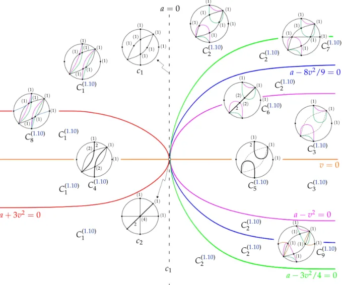
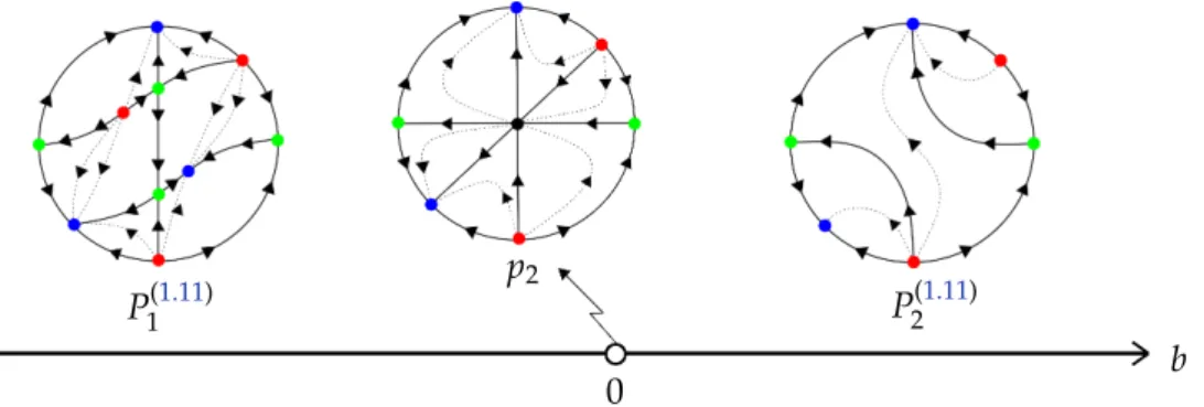
In [18] the authors proved that there are 162 distinct configurations and provided necessary and sufficient conditions for a non-degenerate quadratic differential system to have at least one invariant hyperbola and for the realization of each one of the configurations. These conditions are expressed in terms of the coefficients of the systems. They obtained the normal forms for familyQSHand in this paper we study the following 3 normal forms:
˙
x= a−x32 −2xy3
˙
y=4a−3v2−4xy 3 + y
2
3 , where a6=0.
(1.10)
˙
x=−x2 2 − xy
2
˙
y=b− 3xy 2 +y
2
2, whereb6=0.
(1.11) (x˙ =2a+gx2+xy,
˙
y= a(2g−1) + (g−1)xy+y2, where a(g−1)6=0. (1.12) Our first goal in this paper is to do a complete study of these three families of quadratic systems which possess an invariant hyperbola. Our interest is in the geometry of these sys- tems, as expressed in terms of their invariant algebraic curves, in the impact of this geometry on the integrability of these systems, on their phase portraits and in the dynamics of the systems expressed in the bifurcation diagrams of the families we study. Our third goal is to confront our results with the existing results in the literature and bring to light some missing cases in theses other studies which we point out here. Our geometric analysis is done in detail as this is part of a program of collecting data in order to obtain more global results on the familyQSHand its Darboux theory.
Our paper is organized as follows: in Section 2 we give a number of definitions and propositions useful for the other sections. In Sections3, 4, 5we present a complete study of families (1.10), (1.11) and (1.12). The choice of the first two families is motivated by the fact that they do not satisfy all the conditions in the hypothesis of the Christopher–Kooij theorem, here stated in theorem1.15, but the conclusion of the theorem still holds, while the last family does not always posses a first integral and it will provide a counterpoint. In Section 6 we raise some questions, consider the problem of Poincaré for the familyQSH, and make some concluding comments.
2 Preliminaries
The notion of configuration of invariant curves of a polynomial differential system appears in several works, see for instance [26].
Definition 2.1. Consider a real planar polynomial system (1.1) with a finite number of singular points. By aconfiguration of algebraic solutionsof the system we mean a set of algebraic solutions overCof the system, each one of these curves endowed with its own multiplicity and together with all the real singular points of this system located on these curves, each one of these singularities endowed with its own multiplicity.
Definition 2.2. Suppose we have two systems (S1), (S2) in QSH with a finite number of singularities, finite or infinite, a finite set of invariant hyperbolasH1i :h1i(x,y) =0, i=1, . . . ,k of (S1) (respectively H2i : h2i(x,y) = 0, i = 1, . . . ,k of (S2)) and a finite set (which could also be empty) of invariant straight lines L1j : g1j(x,y) = 0, j = 1, . . . ,k0 of (S1) (respectively L2j :g2j(x,y) =0, j=1, . . . ,k0 of(S2)). We say that the two configurationsC1,C2of hyperbolas and lines of these systems are equivalent if there is a one-to-one correspondence Φh between the hyperbolas of C1 andC2 and a one-to-one correspondenceΦl between the lines ofC1 and C2 such that:
(i) the correspondences conserve the multiplicities of the hyperbolas and lines (in case there are any) and also send a real invariant curve to a real invariant curve and a complex invariant curve to a complex invariant curve;
(ii) for each hyperbolaH:h(x,y) =0 ofC1(respectively each lineL:g(x,y) =0)we have a one-to-one correspondence between the real singular points onH(respectively onL) and the real singular points on Φh(H) (respectively Φl(L)) conserving their multiplicities, their location on branches of hyperbolas and their order on these branches (respectively on the lines);
(iii) Furthermore, consider the total curvesF1 : ∏H1i(X,Y,Z)∏G1j(X,Y,Z)Z = 0 (respec- tively F2 : ∏Hi2(X,Y,Z)∏G2j(X,Y,Z)Z= 0) where Hi1(X,Y,Z) =0, G1j(X,Y,Z) =0 (respectively Hi2(X,Y,Z) =0, G2j(X,Y,Z) =0) are the projective completions ofH1i, L1j (respectively Hi2, L2j). Then, there is a one-to-one correspondence ψ between the sin- gularities of the curves F1 andF2 conserving their multiplicities as singular points of these (total) curves.
It is important to assume that systems (1.3) are non-degenerate because otherwise doing a time rescaling, they can be reduced to linear or constant systems. Under this assumption all the systems inQSHhave a finite number of finite singular points.
In the family QSH we also have cases where we have an infinite number of hyperbolas.
In these cases, by a Jouanolou result (see Theorem 1.5 on page 3), we have a rational first integral.
In [18] the authors classified the familyQSH, according to their geometric properties en- coded in the configurations of invariant hyperbolas and invariant straight lines which these systems possess. If a quadratic system has an infinite number of hyperbolas then the system has a finite number of invariant affine straight lines (see [1]). Therefore, we can talk about equivalence of configurations of the invariant affine lines associated to the system. Given two such
configurationsC1l andC2l associated to systems(S1)and(S2)of (1.1), we say they areequiva- lentif and only if there is a one-to-one correspondenceΦbetween the lines ofC1l andC2lsuch that:
(i) the correspondence preserve the multiplicities of the lines and also sends a real (respec- tively complex) invariant line to a real (respectively complex) invariant line;
(ii) for each line L : g(x,y) = 0 we have a one-to-one correspondence between the real singularities onLand the real singularities onΦpreserving their multiplicities and their order on the lines.
Definition 2.3 ([18]). Consider two systems (S1) and (S2)in QSH each one with an infinite number of invariant hyperbolas. Consider the configurationsC1l andC2l of invariant affine straight lines L1j : g1j(x,y) = 0 where j = 1, 2, . . . ,k of system (S1) and respectively L2j : g2j(x,y) = 0 where j= 1, 2, . . . ,k of system (S2). We say that the two configurationsC1l and C2l are equivalent with respect to the hyperbolas of the systems if and only if:
(i) they are equivalent as configurations of invariant lines, and
(ii) taking any hyperbola H1 : h1(x,y) = 0 of (S1) and any hyperbola H2 : h2(x,y) = 0 of (S2), then we must have a one-to-one correspondence between the real singularities of system (S1) located on H1 and of real singularities of system (S2) located on H2, preserving their multiplicities, their location and order on branches.
Furthermore, consider the curves F1 : ∏h1(x,y)∏g1j = 0 and F2 : ∏h2(x,y)∏g2j = 0.
Then, we have a one-to-one correspondence between the singularities of the curve F1 with those in the curveF2 preserving their multiplicities as singularities of these curves.
The definition above is independent of the choice of the two hyperbolasH1 :h1(x,y) = 0 of(S1)andH2:h2(x,y) =0 of(S2).
Suppose that a polynomial differential system has an algebraic solution f(x,y) =0 where f(x,y)∈C[x,y]is of degreengiven by
f(x,y) =c0+c10x+c01y+c20x2+c11xy+c02y2+· · ·+cn0xn+cn−1,1xn−1y+· · ·+c0nyn, with ˆc= (c0,c10, . . . ,c0n)∈CN whereN = (n+1)(n+2)/2. We note that the equation
λf(x,y) =0, λ∈ C∗ =C− {0}
yields the same locus of complex points in the plane as the locus induced by f(x,y) = 0.
Therefore, a curve of degreenis defined by ˆcwhere
[cˆ] = [c0 :c10:· · · :c0n]∈ PN−1(C).
We say that a sequence of curves fi(x,y) = 0, each one of degree n, converges to a curve f(x,y) = 0 if and only if the sequence of points [ci] = [ci0 : ci10 : · · · : ci0n] converges to [cˆ] = [c0:c10 :· · ·:c0n]in the topology ofPN−1(C).
We observe that if we rescale the timet0 =λtby a positive constantλthe geometry of the systems (1.1) (phase curves) does not change. So for our purposes we can identify a system (1.1) of degreenwith a point
[a0:a10:· · · :a0n:b0 :b10:· · ·:b0n]∈SN−1(R) whereN = (n+1)(n+2).
Definition 2.4.
(1) We say that an invariant curve
L: f(x,y) =0, f ∈C[x,y]
for a polynomial system (S) of degree n has geometric multiplicity m if there exists a sequence of real polynomial systems(Sk)of degreenconverging to(S)in the topology ofSN−1(R)whereN= (n+1)(n+2)such that each(Sk)has m distinct invariant curves
L1,k : f1,k(x,y) =0, . . . ,Lm,k : fm,k(x,y) =0
over C, deg(f) = deg(fi,k) =r, converging to L ask → ∞, in the topology of PR−1(C), with R= (r+1)(r+2)/2 and this does not occur form+1.
(2) We say that the line at infinity
L∞ : Z=0
of a polynomial system (S) of degree n has geometric multiplicity m if there exists a sequence of real polynomial systems(Sk)of degreenconverging to(S)in the topology of SN−1(R)where N = (n+1)(n+2) such that each (Sk) hasm−1 distinct invariant lines
L1,k : f1,k(x,y) =0, . . . ,Lm−1,k : fm−1,k(x,y) =0
overC, converging to the line at infinityL∞ ask→∞, in the topology ofP2(C)and this does not occur for m.
Definition 2.5 ([9]). LetCm[x,y]be the C-vector space of polynomials inC[x,y] of degree at most m and of dimension R = (2+2m). Let{v1,v2, . . . ,vR}be a base ofCm[x,y]. We denote by MR(m)theR×Rmatrix
MR(m) =
v1 v2 . . . vR
χ(v1) χ(v2) . . . χ(vR) ... ... . .. ... χR−1(v1) χR−1(v2) . . . χR−1(vR)
, (2.1)
where χk+1(vi) = χ(χk(vi)). The mth extactic curve of χ, Em(χ), is given by the equation detMR(m) =0. We also callEm(χ)themth extactic polynomial.
From the properties of the determinant we note that the extactic curve is independent of the choice of the base ofCm[x,y].
Theorem 2.6 ([20]). Consider a planar vector field(1.2). We have Em(χ) =0andEm−1(χ) 6= 0 if and only ifχadmits a rational first integral of exact degree m.
Observe that if f = 0 is an invariant algebraic curve of degree m of χ , then f divides Em(χ). This is due to the fact that if f is a member of a base of Cm[x,y], then f divides the whole column in which f is located.
Definition 2.7 ([9]). We say that an invariant algebraic curve f = 0 of degree m ≥ 1 has algebraic multiplicityk if detMR(m)6= 0 andk is the maximum positive integer such that fk divides detMR(m); and it has no defined algebraic multiplicity if detMR(m)≡0.
Definition 2.8 ([9]). We say that an invariant algebraic curve f = 0 of degree m ≥ 1 has integrable multiplicitykwith respect toχif kis the largest integer for which the following is true: there arek−1 exponential factors exp(gj/fj), j = 1, . . . ,k−1, with deggj ≤ jm, such that eachgj is not a multiple of f.
In the next result we see that the algebraic and integrable multiplicity coincide if f =0 is an irreducible invariant algebraic curve.
Theorem 2.9 ([16]). Consider an irreducible invariant algebraic curve f = 0of degree m ≥ 1of χ.
Then f has algebraic multiplicity k if and only if the vector field (1.2) has k−1 exponential factors exp(gj/fj), where(gj,f) =1and gj is a polynomial of degree at most jm, for j=1, . . . ,k−1.
In [9] the authors showed that the definitions of geometric, algebraic and integrable mul- tiplicity are equivalent when f = 0 is an irreducible invariant algebraic curve of vector field (1.2).
In order to use the infinity ofR2as an additional invariant curve for studying the integra- bility of the vector field χ, we need the Poincaré compactification of the vector field χ. For Z6=0 consider the change of variables
x= 1
Z, y= Y Z the vector fieldχis transformed to
χ=−Z P(Z,Y) ∂
∂Z+ Q(Z,Y)−Y P(Z,Y) ∂
∂Y whereP(Z,Y) =Z2P Z1,YZ
andQ(Z,Y) =Z2Q 1Z,YZ .
We note that Z = 0 is an invariant line of the vector field χ and that the infinity of R2 corresponds to Z = 0 of the vector field χ. So we can define the algebraic multiplicity of Z=0 for the vector fieldχ.
Definition 2.10. We say that the infinity ofχhas algebraic multiplicitykifZ=0 has algebraic multiplicityk for the vector fieldχ; and that it has no defined algebraic multiplicity if Z = 0 has no defined algebraic multiplicity forχ.
Let’s recall the algebraic-geometric definition of an r-cycle on an irreducible algebraic variety of dimensionn.
Definition 2.11. Let V be an irreducible algebraic variety of dimension n over a field K. A cycle of dimensionror r-cycle onV is a formal sum
∑
WnWW
whereW is a subvariety of V of dimensionr which is not contained in the singular locus of V, nW ∈ Z, and only a finite number ofnW’s are non-zero. We call degree of an r-cycle the
sum
∑
W
nW. An(n−1)-cycle is called a divisor.
Definition 2.12. For a non-degenerate polynomial differential systems(S)possessing a finite number of algebraic solutions
F ={fi}mi=1, fi(x,y) =0, fi(x,y)∈C,
each with multiplicityniand a finite number of singularities at infinity, we define the algebraic solutions divisor (also called the invariant curves divisor) on the projective plane,
ICDF =
∑
ni
niCi+n∞L∞
where Ci : Fi(X,Y,Z) =0 are the projective completions of fi(x,y) =0, ni is the multiplicity of the curveCi =0 andn∞ is the multiplicity of the line at infinityL∞ :Z=0.
It is well known (see [1]) that the maximum number of invariant straight lines, including the line at infinity, for polynomial systems of degree n≥2 is 3n.
Proposition 2.13 ([1]). Every quadratic differential system has at most six invariant straight lines, including the line at infinity.
In the case we consider here, we have a particular instance of the divisorICDbecause the invariant curves will be invariant hyperbolas and invariant lines of a quadratic differential system, in case these are in finite number. In case we have an infinite number of hyperbolas we can construct the divisor of the invariant straight lines which are always in finite number.
Another ingredient of the configuration of algebraic solutions are the real singularities situated on these curves. We also need to use here the notion of multiplicity divisor of real singularities of a system, located on the algebraic solutions of the system.
Definition 2.14.
1. Suppose a real quadratic system (1.3) has a non-zero finite number of invariant hyper- bolas
Hi : hi(x,y) =0, i=1, 2, . . . ,k and a finite number of affine invariant lines
Lj : fj(x,y) =0, j=1, 2, . . . ,l.
We denote the line at infinity L∞ : Z = 0. Let us assume that on the line at infinity we have a finite number of singularities. The divisor of invariant hyperbolas and invariant lines on the complex projective plane of the system is the following
ICD= n1H1+· · ·+nkHk+m1L1+· · ·+mlLl+m∞L∞
where ni (respectivelymj) is the multiplicity of the hyperbolaHi (respectivelymj of the lineLj), andm∞is the multiplicity ofL∞. We also mark the complex (non-real) invariant hyperbolas (respectively lines) denoting them by HCi (respectively LCi ). We define the total multiplicity TMof the divisor as the sum∑ini+∑jmj+m∞.
2. The zero-cycle on the real projective plane, of singularities of a quadratic system (1.3) located on the configuration of invariant lines and invariant hyperbolas, is given by
M0CS =r1P1+· · ·+rlPl+v1P1∞+· · ·+vnPn∞
where Pi (respectively Pj∞) are all the finite (respectively infinite) such singularities of the system and ri (respectively vj) are their corresponding multiplicities. We mark the complex singular points denoting them by PiC. We define the total multiplicity TM of zero-cycles as the sum∑iri+∑jvj.
In the family QSH we have configurations which have an infinite number of hyperbolas.
These are of two kinds: those with a finite number of singular points at infinity, and those with the line at infinity filled up with singularities. To distinguish these two cases we define
|Sing∞|to be the cardinality of the set of singular points at infinity of the systems. In the first case we have|Sing∞|=2 or 3, and in the second case|Sing∞|is the continuum and we simply write|Sing∞| = ∞. Since in both cases the systems admit a finite number of affine invariant straight lines we can use them to distinguish the configurations.
Definition 2.15.
(1) In case we have an infinite number of hyperbolas and just two or three singular points at infinity but we have a finite number of invariant straight lines we define
ILD=m1L1+· · ·+mlLl+m∞L∞.
(2) In case we have an infinite number of hyperbolas, the line at infinity is filled up with singularities and we have a finite number of affine lines, we define
ILD=m1L1+· · ·+mlLl.
Suppose we have a finite number of invariant hyperbolas and invariant straight lines of a system(S)and that they are given by equations
fi(x,y) =0, i∈ {1, 2, . . . ,k}, fi ∈C[x,y].
Let us denote by Fi(X,Y,Z) = 0 the projection completion of the invariant curves fi = 0 in P2(C).
Definition 2.16. The total invariant curve of the system(S)inQSH, onP2(R), is the curve T(S) =
∏
i
Fi(X,Y,Z)Z=0.
In case one of the curves is multiple then it will appear with its multiplicity.
For example, if a system(S)admits an invariant hyperbola h(x,y)with multiplicity two and the line at infinity Z = 0 has multiplicity one, then the total invariant curve of this system is
T(S) = H(X,Y,Z)2Z=0
whereH(X,Y,Z) =0 is the projection completion ofh=0. The degree of T(S)is 5.
The singular points of the system (S)situated on T(S) are of two kinds: those which are simple (or smooth) points ofT(S)and those which are multiple points of T(S).
Remark 2.17. To each singular point of the system we have its associated multiplicity as a singular point of the system. In addition, when these singular points are situated on the total curve, we also have the multiplicity of these points as points on the total curveT(S). Through
a singular point of the systems there may pass several of the curvesFi =0 andZ=0. Also we may have the case when this point is a singular point of one or even of several of the curves in case we work with invariant curves with singularities. This leads to the multiplicity of the point as point of the curveT(S). The simple points of the curve T(S)are those of multiplicity one. They are also the smooth points of this curve.
Definition 2.18. The zero-cycle of the total curveT(S)of system(S)is given by M0CT =r1P1+· · ·+rlPl+v1P1∞+· · ·+vnPn∞
wherePi(respectivelyPj∞) are all the finite (respectively infinite) singularities situated onT(S) andri (respectivelyvj) are their corresponding multiplicities as points on the total curveT(S). We define the total multiplicity TM of zero-cycles of the total invariant curve as the sum
∑iri+∑jvj.
Remark 2.19. If two curves intersects transversally, this point will be a simple point of inter- section. If they are tangent, we would have an intersection multiplicity higher than or equal to two.
Definition 2.20([24]). Two polynomial differential systemsS1andS2are topologically equiv- alent if and only if there exists a homeomorphism of the plane carrying the oriented phase curves of S1to the oriented phase curves of S2and preserving the orientation.
To cut the number of non equivalent phase portraits in half we use here another equiva- lence relation.
Definition 2.21. Two polynomial differential systemsS1andS2are topologically equivalent if and only if there exists a homeomorphism of the plane carrying the oriented phase curves of S1to the oriented phase curves ofS2, preserving or reversing the orientation.
We use the notation for singularities as introduced in [2] and [3]. We say that a singular point iselementalif it possess two eigenvalues not zero;semi-elementalif it possess exactly one eigenvalue equal to zero and nilpotent if it posses two eigenvalues zero. We call intricate a singular point with its Jacobian matrix identically zero.
We will place first the finite singular points which will be denoted with lower case letters and secondly we will place the infinite singular points which will be denoted by capital letters, separating them by a semicolon ’;’.
In our study we will have real and complex finite singular points and from the topological viewpoint only the real ones are interesting. When we have a simple (respectively double) complex finite singular point we use the notation©(respectively©(2)).
For the elemental singular points we use the notation ’s’, ’S’ for saddles, ’n’, ’N’ for nodes,
’f’ for foci and ’c’ for centers.
Non-elemental singular points are multiple points. Here we introduce a special notation for the infinity non-elemental singular point. We denote by (ab) the maximum number a (re- spectivelyb) of finite (respectively infinite) singularities which can be obtained by perturbation of the multiple point. For example, when we have a non-elemental point at infinity obtained by the coalescence from a node at infinite with a saddle at infinite we will denoted it by(02)SN.
The semi-elemental singular points can either be nodes, saddles or saddle-nodes (finite or infinite). If they are finite singular points we will denote them by ’n(2)’, ’s(2)’ and ’sn(2)’,
respectively and if they are infinite singular points by ’(ab)N’, ’(ab)S’ and ’(ab)SN’, where (ab) in- dicates their multiplicity. We note that semi-elemental nodes and saddles are respectively topologically equivalent with elemental nodes and saddles.
The nilpotent singular points can either be saddles, nodes, saddle-nodes, elliptic-saddles, cusps, foci or centers. The only finite nilpotent points for which we need to introduce notation are the elliptic-saddles and cusps which we denote respectively by ’es’ and ’cp’.
The intricate singular points are degenerate singular points. It is known that the neigh- bourhood of any singular point of a polynomial vector field (except for foci and centers) is formed by a finite number of sectors which could only be of three types: parabolic (p), hyper- bolic (h) and elliptic (e) (see [12]). In this work we have the following finite intricate singular points of multiplicity four described according their sectoral decomposition:
• hpphpp(4)
• phph(4)
• epep(4)
The degenerate systems are systems with a common factor in the polynomials defining the system. We will denote this case with the symbol . The degeneracy can be produced by a common factor of degree one which defines a straight line or a common quadratic factor which defines a conic. In this paper we have just the first case happening. Following [2] we use the symbol [|]for a real straight line.
Moreover, we also want to determine whether after removing the common factor of the polynomials, singular points remain on the curve defined by this common factor. If some singular points remain on this curve we will use the corresponding notation of their various kinds. In this situation, the geometrical properties of the singularity that remain after the removal of the degeneracy, may produce topologically different phenomena, even if they are topologically equivalent singularities. So, we will need to keep the geometrical information associated to that singularity.
In this study we use the notation ( [|];nd)which denotes the presence of a real straight line filled up with singular points in the system such that the reduced system has a node nd on this line where nd is a one-direction node, that is, a node with two identical eigenvalues whose Jacobian matrix cannot be diagonal.
The existence of a common factor of the polynomials defining the differential system also affects the infinite singular points.
We point out that the projective completion of a real affine line filled up with singular points has a point on the line at infinity which will then be also a non-isolated singularity.
There is a detailed description of this notation in [2]. In case that after the removal of the finite degeneracy, a singular point at infinity remains at the same place, we must denote it with all its geometrical properties since they may influence the local topological phase portrait. In this study we use the notation(02)SN,( [|];∅)that means that the system has at infinity a saddle- node, and one non-isolated singular point which is part of a real straight line filled up with singularities (other that the line at infinity), and that the reduced linear system has no infinite singular point in that position. See [2] and [3] for more details.
In order to distinguish topologically the phase portraits of the systems we obtained, we also use some invariants introduced in [25]. LetSC be the total number of separatrix connec- tions, i.e. of phase curves connecting two singularities which are local separatrices of the two singular points. We denote by
• SCff the total number ofSCconnecting two finite singularities,
• SC∞f the total number ofSCconnecting a finite with an infinite singularity,
• SC∞∞ the total number ofSCconnecting two infinite.
Agraphic as defined in [13] is formed by a finite sequence of singular points r1,r2, . . . ,rn (with possible repetitions) and non-trivial connecting orbitsγi fori=1, . . . ,nsuch thatγi has ri as α-limit set andri+1as ω-limit set fori <n andγnhasrn asα-limit set andr1 asω-limit set. Also normal orientationsnj of the non-trivial orbits must be coherent in the sense that if γj−1 has left-hand orientation then so does γj. A polycycleis a graphic which has a Poincaré return map.
A degenerate graphic is a graphic where it is also allowed that one or several (even all) connecting orbitsγi can be formed by an infinite number of singular points. For more details, see [13].
3 Geometric analysis of family (1.10)
Consider the family
(1.10)
x˙ = a− x
2
3 −2xy 3
˙
y=4a−3v2−4xy 3 + y
2
3 , where a6=0.
This is a two parameter family depending on (a,v) ∈ (R\{0})×R. We display below the full geometric analysis of the systems in this family, which is endowed with at least three invariant algebraic curves. In the generic situation
av(a−v2)(a−3v2/4)(a+3v2)(a−8v2/9)6=0 (3.1) the systems have only two invariant lines J1 and J2 and only two invariant hyperbolas J3 and J4with respective cofactorsαi, 1≤i≤4 where
J1=−3p
−a+v2−x+y, α1=p−a+v2− x3 +y3, J2=3p
−a+v2−x+y, α2=−p−a+v2− x3+ y3, J3=−3a+3vx−x2+xy, α3=−v−2x3 − y3,
J4=−3a−3vx−x2+xy, α4=v− 2x3 − y3.
We see that since the number of invariant curve is four, these systems are Darboux inte- grable. We note that ifv=0 then the two hyperbolas coincide and we get a double hyperbola.
Also if a= v2 the two lines coincide and we get a double line. So to have four distinct curves we need to put v(a−v2) 6= 0. We inquire when we could have an additional line. Calcula- tions yield that this happens when a−3v2/4 = 0. We also inquire when we could have an additional hyperbola. Calculations yield that this happens when (a+3v2)(a−8v2/9) =0.
Straightforward calculations lead us to the tables listed below. The multiplicities of each invariant straight line and invariant hyperbola appearing in the divisor ICD of invariant al- gebraic curves were calculated by using for lines the 1st and for hyperbola the 2nd extactic polynomial, respectively.
(i) av(a−v2)(a−3v2/4)(a+3v2)(a−8v2/9)6=0.
Invariant curves and cofactors Singularities Intersection points
J1= −3√
−a+v2−x+y J2=3√
−a+v2−x+y J3= −3a+3vx−x2+xy J4= −3a−3vx−x2+xy α1=√
−a+v2− x3+ y3 α2=√
−a+v2− x3+ y3 α3=−v−2x3 −y3 α4=v−2x3 − y3
P1=(−v−√
v2−a,−v+2
√
v2−a) P2=(v−
√
v2−a,v+2
√
v2−a) P3=(−v+
√
v2−a,−v−2
√
v2−a) P4=(v+
√
v2−a,v−2
√
v2−a)
P1∞ = [0 : 1 : 0] P2∞ = [1 : 1 : 0] P3∞ = [1 : 0 : 0] For v2 >awe have n,s,s,n;N,N,Sifv>0 s,n,n,s;N,N,Sifv<0 For v2 <awe have
©,©,©,©;N,N,S
J1∩J2= P2∞ simple J1∩J3=
P2∞ simple P2 simple J1∩J4=
P2∞ simple P1 simple J1∩ L∞= P2∞ simple J2∩J3=
P2∞ simple P4 simple J2∩J4=
P2∞ simple P3 simple J2∩ L∞= P2∞ simple J3∩J4=
P1∞ triple P2∞ simple J3∩ L∞=
P1∞ simple P2∞ simple J4∩ L∞=
P1∞ simple P2∞ simple
Divisor and zero-cycles Degree
ICD=
J1+J2+J3+J4+L∞ ifv2> a J1C+J2C+J3+J4+L∞ ifv2<a M0CS =
P1+P2+P3+P4+P1∞+P2∞+P3∞if v2 >a P1C+P2C+P3C+P4C+P1∞+P2∞+P3∞if v2 <a T =ZJ1J2J3J4 =0
M0CT =
2P1+2P2+2P3+2P4+3P1∞+5P2∞+P3∞ ifv2 >a 3P1∞+5P2∞+P3∞ ifv2 <a
5 5 7 7 7 17
9 where the total curveThas
1) only two distinct tangents atP1∞, but one of them is double and 2) five distinct tangents atP2∞.
First integral Integrating Factor
General I = J1λ1J2−λ1J
λ1
√
v2−a v
3 J−
λ1
√
v2−a v
4 R= J1λ1J2−λ1−2J
(λ1+1)
√
v2−a
v −1
3 J−
(λ1+1)
√
v2−a
v −1
4
Simple
example I = JJ1
2
J3
J4
√
v2−a
v R= J 1
1J2J3J4