Analysis of Epidemics
J . E. VAN DER P L A N K
Division of Phnt Pathology, Dept. of Agriculture, Pretoria, Union of South Africa
I. Introduction 230 A. Aim of the Chapter 230
B. Some Common Misconceptions 230 C. Epidemics as a Matter of Balance between Opposing Processes . . 231
II. The Multiplication of Infections 232 A. Multiplication within a Crop 232 B. Increase of Disease when the Parasite Does Not Spread between the
Host Plants 240 III. The Amount of Inoculum at Its Source in Relation to Epidemics . . 243
A. The Amount of Inoculum and Rate of Multiplication before the Onset 243 B. Some Comments on the Theory of Forecasting Epidemics . . . 245 C. An Epidemiological View of the Problem of Sanitation; the First
Rule of Sanitation 246 D. An Epidemiological View of Breeding for Resistance . . . 247
E. Secondary Epidemics 248 IV. The Spread of Epidemics 250
A. Factors That Affect the Rate of Spread 250
B. Horizons of Infection 251 C. Continuous and Discontinuous Spread of Epidemics . . . . 252
D. The Determination of Gradients; the Scrapping of Equation 12;
Dutch Elm Disease; Potato Blight 253 E. Scales of Distance; a Tie between Multiplication and Spread . . 256
F. Inverse Distance Scales; the Law of Lesion Size . . . . 259 V. Epidemics in Relation to the Abundance and Distribution of Host Plants 260
A. General 260 B. Disease in Susceptible Plants Scattered among Immune Plants . . 261
C. The "Epidemic Point" in Crowding Plants Together . . . . 262 D. Crowd Diseases; Changes in the Relative Importance of Diseases;
a Glimpse of the Future 263 E. The Effect of Making Fields Larger 264
F. The Paradox; in Praise of Large Fields; the Second Rule of Sanitation 267 G. The Reduction of Disease by Farm and Country Planning . . 268 H. Epidemics in Experimental Plots; an Epidemiological View of Field
Experiments in Plant Pathology 270
VI. The Host Plants . 271 A. Conditions for an Epidemic in Annual Crops 271
B. Conditions for an Epidemic in the Annual New Growth of Perennial
Crops 273 229
C. Epidemics of Disease in Perennial Tissues 274
D. Epidemics of Systemic Disease 278 E. Effect of Genetic Variability of the Host 280
F. Vulnerability and Resistance of the Host to Disease; a Matter of
Natural Selection 283 Appendix: A Suggestion for the Control of Stem Rust of Wheat 284
References 287
I. INTRODUCTION
A. Aim of the Chapter
This chapter is analytical rather than descriptive. In conformity with the basic purpose of this treatise the chapter aims at an understanding of the factors and processes that go to make an epidemic, and not at a description of important epidemics, past or present.
B. Some Common Misconceptions
It is stated in the literature that for an epidemic to occur there must be an aggressive parasite that multiplies fast, spreads far and swiftly, and is not particularly selective in its requirements. These are total miscon
ceptions. They are the cause of much confused thinking and must be disposed of forthwith.
Consider swollen shoot of cacao, a systemic virus disease in West Africa, as an example. The virus complex is carried by slow-moving flightless mealy bugs of the family Pseudococcidae, and spreads largely from tree to tree in contact (Posnette, 1953). It is delicate, and survives for less than an hour in the feeding vectors (Posnette, 1953). The num
ber of infected trees on a farm multiplies slowly; under conditions of unrestricted natural spread it took 30 months for the percentage of infected trees to increase from 31 to 75 (Anonymous, 1949). The spread of infection from farm to farm is also slow. In 1947 the largest area of disease in West Africa had reached a radius of only some 10 miles after having spread continuously since 1922 (Posnette, 1947). Yet there can be no doubt that swollen shoot is a major epidemic. The virus complex is endemic in West African indigenous trees of the Sterculiaceae and Bombacaceae. As a sporadic disease, cacao swollen shoot has a long history in West Africa (Posnette, 1953). But some 30 years ago the epidemic began, with the merging of separate but expanding, more or less circular outbreaks, into larger amorphous areas of dead and dying trees, which spread ever more rapidly and devastated whole farms in their spread (Posnette, 1953). The disease has caused political up
heavals, and the cacao industry from the western Ivory Coast to central Nigeria has needed drastic measures to save it.
Another example is oak wilt, caused by the fungus Ceratocystis fagacearum. The current epidemic of this disease in the United States was rated sufficiently high to get an entire chapter to itself in the limited space of "Plant Diseases," the United States Department of Agriculture's Yearbook for 1953. Yet the parasite has very limited means of spread. It can spread over a distance by some means that are not yet properly understood, but the main spread is from tree to tree. Infection takes place through root grafts, and local barriers such as roads are sometimes enough to stop it (Riker, 1951).
An extreme example is psorosis, a virus disease of citrus. No vector is known. The virus can spread from tree to tree by root grafts, but the natural spread is so slow that it is extremely difficult to demonstrate in orchards. Yet psorosis is currently the greatest killer of citrus trees in California (Moore et al., 1957). Psorosis epidemics, it seems, may take half a century or more to develop.
C. Epidemics as a Matter of Balance between Opposing Processes The human population of a country can increase as a result of a high birth rate; it can also increase as the result of a low death rate. It will increase with a low birth rate provided that the death rate is even lower.
As with men, so it is with plant pathogens. Disease can increase to epidemic levels because (to consider only the extremes) the pathogen has a high birth rate or because it has a low death rate. The miscon- ceptions we have just discussed have arisen because attention has been focused on high birth rate epidemics. But low death rate epidemics are also important, particularly with perennial hosts.
High birth rate epidemics are usually caused by fungi which develop uredospores, conidia, oidia, and the like, and produce local lesions in the host. Low death rate epidemics are caused largely but not entirely by systemic pathogens. The explanation is often fairly obvious. The systemic pathogen is safe within the host, and if the host is perennial and the disease not immediately lethal, a long life of the infected host guarantees a long life to the systemic pathogen. With pathogens as well as with men longevity means a low death rate. The terms are practically equivalent.
The line between the two types of epidemic is often somewhat blurred, but at the extremes the distinction between them is clear and has interesting consequences. High birth rate epidemics are usually con- trolled by fungicides or resistant varieties; low death rate epidemics are mainly controlled by means of sanitation. High birth rate epidemics usually spread fast; low death rate epidemics usually spread slowly.
These and other consequences will unfold themselves logically as we proceed. But the terms high birth rate epidemics and low death rate
epidemics have been used purely to illustrate a point and now will be dropped in favor of more conventional expressions.
II. T H E M U L T I P L I C A T I O N O F INFECTIONS
A. Multiplication within a Crop 1. The Course of an Epidemic
There is no such thing as a typical epidemic. The variety of epidemics in plant pathology is infinite. To mention just two factors, the epidemic varies with the amount of inoculum that is the source of the infection, and this ranges with the different diseases from scarce to abundant; it varies with the rate at which the infections multiply, and this ranges from very slow to very fast. Because of this variety, one example is as good as another. Blight of potatoes, caused by Phytophthora infestans, is chosen here as an example because of its place in the history of plant pathology. But even for this one disease the example we have chosen for illustration is not typical of all epidemics. It is based on data from western Europe. If blight in North America had been the example, stress would have been laid on the danger of epidemics starting from piles of culled potatoes and garbage dumps near towns.
Figure 1 is based on data taken from a probit foliage decay line given by Large (1945) for an epidemic of blight on potatoes in England.
Observations were started on August 11, when 0.1% of the foliage was infected. This is equivalent to an average of about 1 lesion per plant. The epidemic progressed for about 4 weeks, after which all the foliage had been destroyed by blight. The curve that shows this in Fig. 1 is sigmoid.
The figure also shows the rate of increase of infection per cent per day.
The rate for this epidemic began at about 48%, when observations were started on August 11, and gradually dropped to zero as the epidemic ran its course.
In the Netherlands the early history of a potato blight epidemic was studied by van der Zaag (1956). We assume that the results hold for England too. Van der Zaag found that the most important primary foci of infection were infected plants growing from infected seed. These plants had a few weak, shriveled shoots with a few lesions from which spores were released during the second half of May. They were most abundant in the very susceptible variety, Duke of York, in which about 1 primary focus per square kilometer was found. Infection spread first around these foci, then generally over the fields, and from field to field and from variety to variety. Our concern here is not with the progress in any particular field but with the epidemic generally.
These findings show how inadequate a picture Fig. 1 gives of an epidemic. There are 3,000,000 or 4,000,000 plants in 1 sq. km. of potatoes, so that there are (in round figures) 3,000,000 or 4,000,000 lesions per square kilometer of potatoes when 0.1% of the foliage is infected. Still in round figures, infection had to multiply 1,000,000 times from the original foci before the level of 0.1% was reached on August 11. Figure 1 describes the one-thousandfold increase (from 0.1 to 100%) that occurred after
11 Aug. 18 Aug 2 5 Aug. 11 Sept. 18 Sept.
FIG
potatoes e:
1. Lower half: The progress of an epidemic of blight (P. infestans) in (Data of Large, 1945.) Upper half: The increase of infection per day expressed as a percentage of the infection already present.
August 11, and ignores the one-millionfold increase that went before.
And in terms of time Fig. 1 starts in August instead of May, like the biography of a centenarian that starts after his seventieth birthday.
Consider the matter from the farmer's point of view. For him the most important single characteristic of an epidemic is its date of onset. This decides when he must spray or whether he need spray at all. If the date is early—say, in July in England—heavy losses are likely to occur if the disease is unchecked. But if it is late—say, in September—losses are
likely to be small (apart from tuber infection), and spraying would be a waste of material and effort. There are of course some variations in detail (an epidemic may start early and then be checked by a change in the weather) but the general pattern is clear, as can be seen from the analyses of Moore (1943), Large (1952), Beaumont et al (1953), and Large et al (1954). The date of onset is determined by what happens before the onset, i.e., by that portion of the epidemic not described in Fig. 1.
Infection increased one-millionfold between the second half of May and August 11, i.e., in about 80 days. This is equivalent to an average increase "at compound interest" at the rate of 17% per day. But the rate would not have remained at a steady average since it is affected by changes in the weather. Apart from that, the potato becomes more sus
ceptible as it becomes older (Grainger, 1956). One can therefore infer that the rate was considerably less than 17% at the start and increased to 48% by August 11.
2. Rate of Multiplication before the Onset of the Epidemic
For convenience we can define the onset of an epidemic as that time when not more than 5% of the susceptible tissue is infected, or, for systemic diseases, when not more than 5% of the plants are infected.
Within this rough limit we can decide on any criterion we wish; for example, with potato blight in England and Wales the starting point for the assessment of blight is 0.1% infection, and this level can conveniently be taken to indicate the onset.
The rate of increase of disease has been taken as
% = kx(l - χ) (1)
in which k is a constant and χ is the proportion of susceptible tissue that is infected, or, for systemic diseases, the proportion of infected plants. The rate at which infection occurs is, according to this equation, proportional to the product of the proportion of infected tissue and the proportion of healthy susceptible tissue, that is, to the proportion of tissue that is still available for infection. Curves of this equation describ
ing the progress of infection with time have the sigmoid shape so commonly found in plant pathology. Large (1945) applied the equation to blight epidemics and concluded that it would give a good fit to actual blight progress curves within the limits of accuracy of the original observations. Nevertheless the reader is warned that after the onset a good fit can come about only as a result of counterbalancing factors, because the incubation period (i.e., the pre-reproduction period after
infection) inevitably tends to increase the value of k as the epidemic progresses beyond the onset. That is, after the onset, k is just an em
pirical constant even in a constant environment. W e use equation 1 and sigmoid progress curves almost solely to provide a helpful introduction to the study of multiplication. After the introduction the topic is treated in a way that will nearly obviate the need for considering disease progress curves beyond the onset.
Infection is influenced by the weather, the susceptibility of the host, the virulence of the pathogen, etc. So equation 1 will be rewritten in the form
ft = kx{\ - x)f(T#,S . . . ) (2)
in which f ( Γ , H, S . . . ) is a function of the temperature and humidity of the air, the susceptibility of the host, and so on.
Before the onset of an epidemic, χ is small and, in the definition already given for the onset, less than 0.05. As a good approximation for the progress of infection up to the onset, the term (1 — x) can be dropped and equation 2 rewritten as
·) (3)
. 0 (4) By definition, r is the rate of increase per cent per day (or per year, if
years are the units of time) up to the onset of the epidemic. Within the limits of the approximation just stated r is independent of the progress of the epidemic (up to the onset) and becomes a direct reflection of the environmental conditions, the susceptibility of the host, and so on. A qualification, normally of minor importance, will be discussed in Sec
tion II, A, 6.
3. Some Comments about r
One must become familiar with r. It is a fundamental and perhaps the most useful concept of epidemiology. It plays its part not only in multiplication rates, but also in the rate of spread of epidemics in dis
tance (Section IV, A and E ) , in the theory of forecasting (Section III, B ) , in sanitation (Section III, C ) , and directly or indirectly, in much else.
The impression may have been given that r is only an approximation.
That is incorrect. For convenience r is allowed to make its debut ap
proximately as the percentage rate of multiplication at or before the
^ = kxf{T,H,S . . _ 100 dx
χ dt
= 100fc/(T,#,S .
onset of an epidemic, which is accurate enough for present purposes.
But r is a concept capable of exact determination (as by equation 5) and applicable throughout the course of the epidemic. The reasons for using it mainly at or before the onset will appear later.
In reporting the results of censuses, human birth rates, death rates, and rates of increase of population are given in terms of 1,000 of popula
tion. It is not assumed that the rates are the same for all hours of the day, for all seasons of the year, or for all years of boom and depression, peace and war. The crude rates are simply a convenient way of ex
pressing what is happening. So too r can be regarded as a convenient way of reporting the results of censuses of infections before or at the onset.
It is not implied that r is constant from hour to hour or day to day.
It just expresses the tempo of developments up to the onset in an uncomplicated way. But one condition is implied: fractions of a day or, if appropriate, a year must be avoided. When, for example, it is calculated in Section III, C that an epidemic would be delayed 3.7 days, this must be interpreted as "from 3 to 4 days."
In one way r has an advantage over crude census rates, which are subject to the influence of varying proportions of the population in the different age groups, particularly to a varying proportion of women of childbearing age. Superficially, the same problem occurs with r. With potato blight, for example, it takes from 4 to 6 days or longer after inoculation for spores to be produced. But for most of this period there is no recognizable lesion, and spore formation begins soon after the lesions become visible in the field. Up to the time of the onset of the epidemic relatively few of the lesions seen in the field are not of spore- bearing age; one could without great difficulty count as lesions only those of an age to produce spores. The validity of using lesions of this sort for determining multiplication rates is examined in Section II, A, 6.
The magnitude of r reflects the effect of temperature, humidity, rain
fall, wind, and other environmental factors on multiplication; it reflects among other factors the resistance or susceptibility of the host, the proportion of spores that germinate, the proportion of germinated spores that manage to enter the host and establish infection, the rate of in
crease in size of the lesion, the speed at which spores are produced and their number, the abundance of vectors and their mobility, efficiency, and distribution, and the size and number per acre of the host plants.
It summarizes the equilibrium of the factors (except χ itself) that affect the tempo of multiplication. Because of this, few of these factors will be specifically dealt with in this chapter. There is, for example, no dis
cussion of the effect of weather and climate. This may seem strange in a chapter on epidemiology. But it is logical. When a forecaster uses his
knowledge of the weather and other relevant factors to forecast an epidemic, he is in fact forecasting a faster rate of multiplication. To him the weather and other factors are important. To us (for the purpose of this chapter) the rate of multiplication is important. This statement carries no implication that the one approach is better than the other.
There are several possible approaches to the discussion of epidemics.
One chooses what one believes to be the most apt for one's purpose.
4. The Estimation of r
Substitute r/100 for kf (T,H,S . . . ) in equation 2, integrate, change logarithms to the base 10, and rearrange thus:
230 . 32(1
-
xt) _Here X i and x2 are the proportion of susceptible tissue infected (or, for systemic diseases, the proportion of infected plants) at dates tx and t2, and t2 — £i is the interval in days (or years, if this is appropriate) be- tween these dates.
For example, according to the data of Large (1945) blight in pota- toes at Dartington in 1942 increased from 0.1 to 5.0% in 7 days. Here
* i and x2 are 0.001 and 0.05, respectively, and t2 — tx is 7 days. From equation 5, r = 57% per day.
In general, the use of equation 5 assumes that the lesions are randomly distributed. In the particular case of potato blight there is the independent evidence of Gregory (1948) that this is so; but randomness is not the rule. There are often quick departures from randomness, especially when systemic diseases multiply, particularly the systemic diseases of trees. There is a general rule about this: the smaller the size of lesion, the higher the value of x2 that can be used without incurring a serious error from lack of randomness. A systemically infected plant must be considered as a single lesion (Section IV, F ) .
As another example, consider cauliflower mosaic. It spreads in non- random fashion to form nests of infected plants (Broadbent, 1957). In a trial with different strains of cauliflower there were 1.7 and 5.9% infected plants on August 21 and September 4, respectively (see Fig. 4 in Broad- bent, 1957), so X i and x2 are 0.017 and 0.059, respectively, and t2 — tx is 14 days; whence r is 9.2% per day. The epidemic was started artificially by planting an infected plant at the center of each plot of 121 plants, so 5.9% infection represents roughly 7 plants around each infector plant. The evidence is that at this stage the error from nonrandomness is small, so the estimate of r is fairly trustworthy; but at much higher values of x2 estimates would be too low.
With local lesion disease on plants that grow between tx and t2, allowance must be made for new susceptible tissue. If susceptible tissue increases m times between tx and t2, equation 5 must be rewritten as
230 , mx2(l — Xi) ,a\
Chester (1943) gives figures for the multiplication of leaf rust (Puccinia triticina) of wheat in Oklahoma. After a severe winter fol
lowed by normal weather, infection increases at a steady rate from 1 pustule per 1,000 leaves at the beginning of March to 10 pustules per leaf at the beginning of June. During this period there is a tenfold increase of leaf tissue (Chester, 1946); hence m is 10. The ratio x2/xx is 10,000, and t2 — f i is 92 days. An infection of 10 pustules per leaf is equivalent to about 1% infection, according to Fig. 13 of Chester (1950);
so x2 is 0.01 and x± is even smaller, and we can ignore the terms (1 — X i ) and (1 — x2). By equation 6, r = 12.5% per day.
5. General Comments on the Restriction of Much of This Chapter to Events before the Onset
Physical chemistry advanced far in the theory of dilute solutions.
The gas laws were applied to dilute solutions, and dissociation constants were determined in dilute solutions. This was done in the first place to avoid the difficulties of dealing in theory and practice with the behavior of molecules and ions at high concentrations. In the same way this chapter deals to a great extent with the theory of dilute concentrations of disease: of disease up to the onset, defined arbitrarily as the 5% level.
Primarily the reason for this is to avoid the objection against using dis
ease progress curves after the onset.
How much information do we lose by confining quantitative discus
sions to the period up to the onset? The answer is: surprisingly little. Con
sider these examples. In Section III, C an equation is given that evaluates sanitation in terms of a delay in the onset of the epidemic. If the weather and other conditions stay constant, the delay in the onset is also the delay in reaching the 50% level of disease or the 99% level. If the weather changes, then interest is changed from the factor of sanitation to the factor of weather. By describing the effect of sanitation on the onset, one has in effect described all that needs to be described about the effect of sanitation on the course of the epidemic. In other words, the loss of information from confining attention to the period up to the onset is negligible. Also, it does not matter what criterion one takes for the onset, provided that it is not more than about 5%; it could just as well or better be taken at 0.1%. In Section III, Β we discuss the application
of r to the theory of forecasting; in most cases forecasts are in practice confined to the onset of an epidemic.
Gradients of infection away from the source figure largely in Sections IV and V. With gradients, too, it can be shown both that it is wise to keep calculations to the period up to the onset of the epidemic and that remarkably little information is lost by doing so. In this chapter we do in fact discuss gradients at higher levels of disease, and correct the data as best we can. But this is only through lack of choice; the data are so scant that one cannot at present afford to be selective.
6. Justification for Using the Law of Compound Interest When There Is an Incubation Period
The meaning given to r is that it is the rate of compound interest (per cent) up to the onset. True compound interest (we are not con
cerned with bankers' compound interest) is added to accumulated cap
ital as it is earned, and then instantly begins earning itself; the concept of an incubation (i.e., pre-reproduction) period is foreign to the law of compound interest as it is used in science. Are we then justified in applying the law, as represented by r, to plant disease? It seems that we are, and it will be shown that r can be used as an apparent rate.
The meaning of χ is the proportion of infected tissue in which incu
bation is complete. The infection is visible and the lesions are of an age to produce inoculum (according to the suggestion in Section II, A, 3 ) . Consider now the total proportion x? of tissue that is infected, even if incubation is still incomplete. To simplify the argument, we shall con
fine attention to events before the onset of the epidemic. Instead of equations 3 and 4, let us write for the same set of observations
dx' r f , .
Here x^t-p is the proportion of infected tissue at time t — P, in which Ρ is the incubation period. It is the proportion of tissue in which incuba
tion is complete and therefore has the same meaning as χ in the earlier equations. It can be determined that
Pr
r = r'e 1 0 0' (8)
In effect, r is a compound interest rate to which Ρ contributes, out
wardly like any other factor, such as the abundance of vectors.
Equation 8 holds only when Ρ and κ* are constant. More generally, it can be shown that despite an incubation period the concept of compound interest is valid even if Ρ and f vary with temperature, humidity, etc.
There is more to it than just that. In the early history of an epidemic
(for example, soon after inoculation in an artificial epidemic) r at first varies with time, even if Ρ and r9 are constant, and only later settles down to the stable value given by equation 8. The larger the product Pr, the larger are the variations. Similar variations occur when, for example, an epidemic is checked by drought and then builds up again.
The previous history of the epidemic, every previous fluctuation, is remembered in the multiplication rate, and this memory factor is the special contribution of an incubation period to the concept of com
pound interest.
There is a qualification. Previous memory is wiped out each time multiplication stops for a continuous interval at least as long as P, and then starts anew. Hence, the memory factor can cause a drift in the multiplication rate of potato blight from day to day, but not in that of potato leaf roll from year to year.
Variations in the value of r, whether caused by memory or any other factor, are properly cared for by equation 5. This equation estimates the average of the value of r at every instant between any times t1 and t2, irrespective of any variations that occur.
But although it is important to know that the memory factor's effect on r is correctly estimated, it is often equally important to know how to eliminate this effect so that other factors can be studied without inter
ference. Except within approximately 2.2 Ρ days after inoculation in an artificial epidemic or 1.2 Ρ days after the end of a major interruption in a natural epidemic, the effect of the memory factor on r can be made small by arranging that the interval between tx and t2 should be as near to 1.2 Ρ days (or a multiple thereof) as is possible without using frac
tions of a day. For example, if Ρ is 6 days and it is wished to study in an artificial epidemic the separate effect on r of factors other than the memory factor, observations should begin whenever convenient after the thirteenth day from inoculation and then be made at weekly inter
vals. Very exact knowledge of Ρ is here unnecessary, and in the example just quoted an 8-day interval between tx and t2 would also almost elim
inate the memory factor's effect on r.
B. Increase of Disease when the Pathogen Does Not Spread between the Host Plants
Consider bunt of wheat caused by Tilletia caries and T. foetida.
Plants are infected as young seedlings, and do not release spores until the grain has been formed. One plant cannot infect another during the course of the season. There is multiplication of infection, but only as an increase from season to season and not within a single crop. Many other systemic smut fungi behave similarly.
With obligate heteroecism there are similar restrictions. The apple rust fungi Gymnosporangium spp. move hither and thither from apples to the alternate hosts and back. During this movement from one host to the other there can be a multiplication of infection, but there is no multiplication directly from apple to apple. Similarly, Cronartium ribi- cola does not spread from pine to pine.
With many of the systemic or quasi systemic vascular wilt diseases the pathogen is not returned in great quantity to the soil until the host dies. The pathogen may build up from season to season, but it does not spread much from plant to plant during the season.
Sometimes there is apparently no spread from plant to plant and no building-up within the host species even over the seasons. Eastern X virus spreads from chokecherry (Prunus virginiana) to peach but ap- parently not from peach to peach (Hildebrand, 1953). The virus of Pierce's disease has a wide range of species of host plants from which it infects grapevines, but it does not seem to spread from grapevine to grapevine (Hewitt et al., 1949). Tomato spotted wilt virus infects tobacco, but the thrips vectors do not breed on this host and there is no evidence of spread from tobacco to tobacco (van der Plank and An- derssen, 1945). Peaches with X disease, grapevines with Pierce's disease, and tobacco with tomato spotted wilt apparently do not contribute to the building-up of an epidemic of these three virus diseases; in them epidemics are secondary (see Section III, D ) and are the result of multi- plication in other hosts.
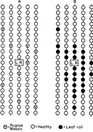
Absence of spread from plant to plant can occur at times even with diseases that normally spread. Figure 2A, reproduced from a report by Doncaster and Gregory (1948), shows the distribution of rugose mosaic, caused by virus Y, in an isolated potato field. This field was initially free from virus Y, but was invaded from a source 300 yd. away. The plants which were infected as a result of this invasion did not pass the infec- tion on to their neighbors, and there was no evidence of secondary spread. Absence of secondary spread can be expected when the invasion takes place late in the season or when the presence of vectors is transient. It is possibly not uncommon.
The type of increase without multiplication which has been discussed in the previous five paragraphs can cause an epidemic which super- ficially resembles other epidemics but which is fundamentally distinct.
There is, for example, no reason why the progress curve of the epidemic with time should be sigmoid. Often the approach to control is different.
It is therefore important to be able to detect when infection is increasing without spreading from plant to plant.
This can be done in various ways. One can mark infected plants and
determine whether they are foci of infection by comparing the number of plants which become infected in an area near them with the number of plants which become infected in a comparable area at a distance away from them. But the most convenient methods use the distribution of
A Β
®=M o f a !c O-Healthy # = L e a f roll
FIG. 2. Distribution of rugose mosaic and leaf roll around an infected plant, L.R., grown from a potato tuber infected with leaf roll. For convenience, rugose mosaic and leaf roll are shown in separate diagrams, A and B, respectively. (After Doncaster and Gregory, 1948).
diseased plants in the field or orchard without a knowledge of their history. Figure 2B shows how leaf roll develops in a potato field around an infected plant grown from an infected tuber. There is a nest of diseased plants near this plant. Nests of this sort vary in their compact
ness and shape from disease to disease, but it is probably safe to assume that with all plant diseases there is a tendency for infected plants to aggregate to some extent near the source of infection. (The tendency is greatest when f is low in value and the gradients are steep;
see Section IV, Ε and F about scales of distance.) The test for spread of
infection is a test for aggregations. Cochran (1936) examined some gen
eral tests, and Todd (1940) and Freeman (1953) developed a test for the special case of the death of trees planted at the corners of a square lattice in a rectangular plantation. The simplest test yet devised makes use of doublets (van der Plank, 1946). A doublet consists of 2 adjacent diseased plants. If η plants are examined in sequence, and of these μ are diseased, the expected number of doublets is
ά = \μ{μ~ 1). (9)
A run of 3 diseased plants is counted as 2 doublets; a run of 4, as 3 doublets; and so on. A test of significance has been worked out by G. A.
Mclntyre of the Commonwealth Scientific and Industrial Research Or
ganisation, Canberra, Australia, and it is hoped it will be published shortly.
As an example, the distribution of leaf-roll-infected potato plants in Fig. 2B is analyzed. There is a total of 100 plants, including the original diseased plant; of these, 28 are infected. If one starts at the top left corner, reads down the first row, up the next, and so on, one counts 19 doublets. The expected number is only 28 X 27/100 or 7.56. The infected plants show excessive (nonrandom) aggregation. A corres
ponding analysis for the 9 potato plants with rugose mosaic in Fig. 2A gives d (observed) 0 and d (expected) 0.72. There is no evidence of nonrandom aggregation. In practice one is usually concerned with col
lecting evidence for the absence rather than for the presence of spread of infection. Extensive data are needed, and precautions must be taken against extraneous heterogeneity of the field. The method can be used to examine evidence for spread in any direction, and counting can start from any randomly chosen starting point. Missing plants, uneven spac- ings, or changing directions do not affect the analysis mathematically, although they may affect its interpretation biologically. From what is written in Section IV, F it follows that spread of infection is most easily detected by this method if the disease is a systemic disease of trees.
III. T H E A M O U N T O F I N O C U L U M A T ITS SOURCE I N R E L A T I O N TO E P I D E M I C S
A. The Amount of Inoculum and Rate of Multiplication before the Onset In the preceding section our concern was with rates of multiplication.
The amount of inoculum at the source of the epidemic must now be considered. When infected plants are the starting inoculum—when, for example, epidemics of potato blight start from lesions on infected shoots developing from infected tubers or when potato leaf roll spreads from an
infected plant, the sequence of multiplication is homogeneous. Lesions produce lesions, and infected plants produce infected plants. We shall be concerned only with homogeneous sequences. When the source of inoculum is resting spores or anything but infected plants, we consider the sequence as starting from the first plants to be infected directly from this inoculum, i.e., the first infected plants are considered as the inoculum at its source. This restriction to homogeneous sequences simplifies what has to be discussed without affecting the conclusions appreciably.
Suppose J0 and ί are respectively the amounts of inoculum (in terms of the number of lesions or, for systemic diseases, the number of infected plants) at the source and at the onset of the epidemic which was defined in Section II, A, 2.
/ = J0e ^1 0 0. (10)
Here t is the time taken up to the onset, and r has the meaning given in earlier equations. To quote an example given previously, if P. infestans multiplies a millionfold in 80 days,
e80r/100 = 7//0 = 1 Q6
whence r = 17.3% per day. This is an average rate for the 80 days.
More often one needs to know the effect of a change in the amount of inoculum at the source: a change brought about, for example, by sanitation. One can therefore profitably rewrite equation 10. Suppose the amount of inoculum at the source is reduced from J0 to J'0. The delay in the onset of the epidemic, At, can then be determined from the equation
70 = / ΝΔ< /100
whence
230, Jo
Δ < = — togyr- (11)
' J- 0
In the equation, r is the rate during the time of the delay. Logarithms are to the base 10.
Suppose r = 69.3% per day at the onset. How long will the onset be delayed by halving the amount of inoculum at its source?
230 log 2 69.3
= 230 X 0.301 69.3
= 1.0.
The answer is 1 day. Natural compound interest of 69.3% per day, which is added to the accumulated capital at every instant, is equal to 100%
"banker's" compound interest, which is added once a day. This numerical problem makes the obvious point that if the amount of infection is doubled every day, halving the amount at its source will postpone the onset by a day. The criterion for the onset must of course be fixed, but, provided that it is fixed within the limit stated in Section II, A, 2, the particular value at which it is fixed has no relevance. (But read also Section II, A, 5.)
Consider another example. Broadbent (1957) tested the use of barriers to protect cauliflower seedlings from mosaic, and found that a barrier of three rows of barley around the seedbed reduced infection from 3.0 to 0.6%. How long would the onset of an epidemic of cauli- flower mosaic be delayed in crops planted from protected seedbeds?
Use the value r = 9.2% per day, calculated for cauliflower mosaic in Section II, A, 5.
., 2 3 0 , 3.0
M = 9 ^l 0 g0 6
= 17.5.
The onset of the epidemic would be delayed 17.5 days. For properly apt results, r should be measured for the same variety as that used in the barrier experiment, in the same district, at the same time of the year, in the same type of soil, etc.
B. Some Comments on the Theory of Forecasting of Epidemics The method and effectiveness of forecasting epidemics varies with the value of r in equation 11. Consider the two extremes of forecasts that ignore, and forecasts based entirely on, the amount of inoculum at the source.
1. Forecasts That Ignore the Amount of Inoculum
According to equation 11, the higher the value of r at the onset, the less the error of a forecast of the time of onset that ignores differences in the amount of inoculum at the source. If r is large enough, approxi- mate forecasts become possible without reference to inoculum. An alter- native condition would be that the amount of inoculum is so large that it ceases to be a limiting factor. Both conditions possibly exist with, say, apple scab when scabby spring weather follows a fall and a winter favorable to the survival of large amounts of inoculum in dead leaves.
Potato plants become more susceptible to blight as they grow older (Grainger, 1956), and high values of r are possible toward maturity.
It is this fact of a high value toward maturity that makes short-range forecasts of blight feasible on weather data alone. It has been found that there may be a "zero time" a date (July 1 in west Scotland) before which forecasts based on weather data alone are invalid (Grain
ger, 1950). Interpreted by equation 11, "zero time" is the date on which the magnitude of r becomes high enough to blur the effect of variations in the amount of inoculum and make the epidemic specially sensitive to the weather. The more susceptible the variety, the earlier can "zero time" be fixed or, alternatively, if "zero time" is unchanged, the more accurately can forecasts be made.
2. Forecasts Based on the Amount of Inoculum Alone
As the value of r at the onset decreases, the effect of variations in the amount of inoculum on the date of the onset increases. With low enough values of r the importance of the inoculum factor becomes dominant, and approximate forecasts can be based on it alone. The number of sclerotia of Sclerotium rolfsii in the soil can be used to forecast losses of sugar beet from this fungus (Leach, 1938). In general the soil is not a medium conducive to the fast multiplication of pathogens, and methods of forecasting other diseases caused by soil-borne pathogens on inoculum alone are likely to be feasible.
C. An Epidemiological View of the Problem of Sanitation:
the First Rule of Sanitation
Equation 11 tells us that, measured as a delay in the onset of an epidemic, the benefit of a given percentage reduction in the amount of inoculum at its source is inversely proportional to r, the magnitude of r being determined at the time of the delay. This is the first rule of sanitation.
Within the limits of one disease the rule means that sanitation helps most when it is needed least. Before any method of sanitation is recom
mended for the control of a disease, it should be ascertained that the method will remain effective even during seasons when conditions are such that infection multiplies at its fastest.
In comparing different diseases the rule means that control by sani
tation is most apt for those diseases that multiply most slowly. If r is large, sanitation is relatively ineffective, and it is usually necessary to use fungicides or, alternatively, to call in the plant breeder to produce a resistant variety, i.e., to bring down the magnitude of r. When r is small, one is likely to be dealing with a disease that can be controlled by sanitation: by crop rotation, by fumigation of the soil before the crop is planted, by destroying diseased crop residues or using manure
free from inoculum, by planting healthy or disinfected seed and nursery stock, by roguing out diseased plants, by isolating fields from sources of inoculum, by destroying weeds or other hosts that can carry infec
tion, or by any other method that reduces inoculum at its source.
For example, systemic diseases tend to have low values of r, and a study of the literature shows that the majority of them are controlled by sanitation in one form or other.
As r increases, sanitation becomes less effective. But where do we draw the line? At the one extreme, with very low rates of multiplica
tion, sanitation is almost completely effective; for example, on present knowledge, a citrus grower can be protected against losses from psorosis by the sanitary measure of using only healthy nursery stock to plant his orchards. Are there, at the other extreme, infections that multiply so fast that sanitation is worthless? The answer depends on the circum
stances. Consider this example. A field of potatoes grown from blight- free seed can become infected with blight from infected refuse piles or from infected fields. Take the second alternative. From calculations based on meager data in the literature, it can be estimated that doubling the isolation of a potato field from its neighbors would reduce the amount of blight that the field gets from its neighbors by 83%. (See Section IV, Β and D.) If, from Fig. 1, we take r to be 48% per day, this isolation will postpone the onset of an epidemic by 3.7 days. (Here ίο/ί'ο —100/(100-83).) On an allowance of an increase of a ton of tubers per acre per week during the critical period of the growing sea
son, isolation to the extent stated would mean a gain of crop in an unsprayed field of about half a ton per acre. Whether this gain would be worth working for depends on the circumstances. On a small farm, isolation is impossible or possible only at the cost of arrangements that are not acceptable to the farmer. But on a large estate some farm planning with an eye to isolation is not ruled out. It is not for our present purpose desirable to pursue this topic at length, but it should be stated that even with a fast multiplying disease like blight of pota
toes the possibility of sanitation cannot be excluded before conditions are analyzed.
D. An Epidemiological View of Breeding for Resistance One especially important deduction from equation 11—and the first rule of sanitation—concerns resistant varieties. Plant breeders like to aim at high resistance or complete immunity; this is desirable, and the effect of immunity is readily understandable: there is no epidemic (and in that case the matter would be outside the scope of this chapter).
But commonly the available resistance is only partial; infection occurs,
but at a slower rate. The magnitude of r is reduced, and the value of sanitation correspondingly increased. Every quantum of resistance, how
ever small, increases the efficiency of sanitation; and every quantum of sanitation increases the value of the partial resistance. As methods of control, sanitation and partial resistance should go together. When a disease is controlled by sanitation, partial resistance in any measure is an achievement not to be despised. It has been much undervalued in plant pathology, largely as the result of ignoring its connection with sanitation.
Ε. Secondary Epidemics
An epidemic can be defined as secondary if it starts from inoculum derived from another, earlier epidemic. In Section II, Β it was observed that epidemics of eastern X disease of peaches, Pierce's disease of grape
vines, and tomato spotted wilt on tobacco are secondary because there is apparently no spread of the diseases in the crops mentioned. Infection must come from outside.
In the Netherlands van der Zaag (1956) found that with the potato variety Duke of York there was about 1 primary focus of infection per square kilometer at the start of the season, this focus originating from an infected seed tuber. With the more resistant variety Noordeling, primary foci were much rarer or entirely absent. Further, he tested varietal differences by artificially inoculating leaflets in the field before natural infection was apparent, and then 12 days later counting how many leaflets had become secondarily and naturally infected from these primary artificial sources. For every 1 lesion on Noordeling that devel
oped secondarily around the primary source, there were 180 on Duke of York. From this we infer that the magnitude of r was roughly 180 times as great for Duke of York as for Noordeling. This estimate is rough but adequate; the evidence does not allow an exact estimate of either r or f. Epidemics in Duke of York take about a month to develop from the primary foci, so, from equation 11, an epidemic in Noordeling would need 180 months to develop. If one adds to this the information about the scarcity of natural primary foci with Noordeling, the period needed would be much greater. Even if one admits the possibility of error, the differences are striking enough to make it reasonably certain that a primary epidemic of blight in Noordeling is improbable in a growing season limited to 4 or 5 months. If Noordeling becomes sig
nificantly blighted, it is almost certainly as a result of infection obtained initially from some other variety.
The tendency for disease to spread from more to less susceptible varieties and cause secondary epidemics in them, increases with the
extent to which initial inoculum must multiply to cause an epidemic.
For any given time up to the onset, the logarithm of the amount of multiplication is proportional to r. If two varieties differ in that in the one r is twice as great as in the other at all times, then by the time the more susceptible variety has multiplied 102 times the less susceptible will have multiplied 10 times; by the time the more susceptible has multiplied 106 times the less susceptible will have multiplied 103 times.
As multiplication continues, the difference in level of disease between the varieties increases. The more the multiplication needed before a level of, say, 5% is reached, the greater is the difference in disease between the varieties when the more susceptible has reached that level; hence, other things being equal, the greater the chance that disease in the less susceptible variety will be influenced by inoculum from the more sus- ceptible. With diseases like potato blight, in which relatively little inoculum survives the winter, the danger of susceptible varieties starting secondary epidemics in other varieties is correspondingly great.
Late blight, caused by Phytophthora infestans, can survive peren- nially on tomatoes in countries in which tomatoes are grown all the year round. It can also be brought into the summer-grown tomato plants of colder climates by blight-infected transplants imported from warmer areas. But late blight of tomatoes has also a considerable literature of epidemics secondary to those of potatoes. Neighboring blighted potato fields or potato refuse piles are repeatedly implicated as the source of tomato blight. But in one detail there has been a noteworthy change in the literature since Mills (1940) summarized it. In 1940 races of Phytophthora infestans from potato were poorly adapted to tomatoes, and, according to Mills, had to be trained to attack tomatoes by a few passages through tomato leaves. Nowadays there are frequent refer- ences in the literature to potato races that readily attack tomatoes, although a distinction between potato and tomato races still exists. On the general evidence of the literature, secondary epidemics on tomatoes are now more easily established from potatoes. There has been, it would appear, a change in the relationship between P. infestans and the potato, which has also involved the tomato secondarily and possibly incidentally, and which has perhaps been the cause of the destructive epidemics of tomato blight on a scale unknown before 1946.
There is a type of secondary epidemic brought about by mixed cropping. The apple variety Delicious has considerable resistance to powdery mildew, caused by Podosphaera leucotricha. Jonathon is very susceptible and is commonly used as a pollinator for Delicious. In mixed orchards spores from diseased Jonathans may start secondary epidemics on Delicious which are severe enough to require control measures
(Sprague, 1953). Hardwoods grown alone are normally resistant to Fames annosus but may be killed when grown in mixed stands with susceptible conifers in which inoculum builds up (Peace, 1957). These examples show the value of uniformity of resistance in minimizing the risk of secondary epidemics, a point to remember when reading Sections VI, C, 2, f and VI, E .
Secondary epidemics provoked by mixed cropping are often used by plant breeders to eliminate susceptible lines of seedlings. A variety known to be susceptible is interplanted with the material to be sorted out in order to ensure that infection will be present in the breeders' plots. The method is simple and convenient, but there is the danger of confusing the smaller amount of resistance adequate to stop a primary epidemic with the larger amount needed to cope with a secondary epidemic.
IV. T H E SPREAD O F E P I D E M I C S
A. Factors That Affect the Rate of Spread
Section IV describes how an epidemic spreads over a distance. Three factors are considered at the start. A fourth factor, scale of distance, is discussed later in the section.
1. The Gradient of Infection
The probability that a healthy plant in a given direction will become infected depends on the distance of that plant from the source of infec
tion. Infection grades away (usually smoothly, but not necessarily so) from the source. Unless otherwise stated, the source will always be taken to be a point—a single plant, for instance—and not a field or strip.
Gradients should be determined only when the percentage of infection is low; apparent gradients necessarily become flatter as disease mounts.
2. The Abundance and Distribution of Susceptible Host Plants The probability that a spore or other propagule will travel a given distance is proportional to the number of propagules released at the source. If the number of air-borne spores at the source is multiplied 100 times, then on an average 100 times as many as before will blow past the first milestone, 100 times as many past the second, and so on. When heavy spore showers are detected hundreds of miles from the nearest source, it is reasonably certain that the source is not a single plant but fields of plants, not just a few fields but hundreds of acres of fields.
Abundant host plants mean, too, that the leaps the pathogen need make
from one host plant to another are small. Their distribution—whether in small fields or large—also affects the pathogen's spread; this is a matter to be discussed in Section V.
3. The Rate of Multiplication
Spread is multiplication at a distance from the source of inoculum;
and, for a given gradient, multiplication at a distance is related to multiplication in general. Fast multiplication of disease lesions means fast spread of disease. The connection has long been tacitly accepted, and pathologists commonly use the words "multiplication" and "spread"
interchangeably. A tie between multiplication and spread is discussed in Section IV, Ε (equation 1 3 ) .
B. Horizons of Infection
Horizons of infection have been discussed by van der Plank (1949b).
For argument's sake suppose temporarily that the probability that a lesion (or, for systemic diseases, an infected plant) will form a daughter lesion in unit time on a healthy plant at a distance s is
Here a and b are constants. W e shall not bother about the accuracy of this equation; the relationship shown is just scaffolding, which will be removed later. Suppose that there are infected fields scattered over a large area, and consider any field as center. Suppose that this field is only lightly infected: that the epidemic in it has not gone further than the onset, and that it receives inoculum from other fields in a sector narrow enough for the gradients toward the center to be considered uniform. The probability that a lesion will develop in this field as a result of inoculum received from a parent lesion two units of distance away in the sector is l/2& times the probability that a lesion will develop from inoculum from a parent lesion one unit of distance away in the sector. But on an average the number of parent lesions two units of distance away is twice the number one unit away (because for a given angle at the center the arc is proportional to its radius). Hence on an average the number of lesions caused by inoculum received from all sources (all parent lesions) two units away is 2/2& or 1/26*1 times the number from inoculum received from all sources one unit away. Sim
ilarly the number from inoculum received from all sources three units away is 1 / 3& 1 times the number from all sources one unit away. If Q is the number of lesions from inoculum received from all sources one unit
of distance away the number of lesions from inoculum received from all sources at all distances is
If b > 2, this series is convergent, and there will be a limit from beyond which inoculum will not come.
To simplify calculations, suppose that the distance between fields is relatively large and that the fields are uniformly infected and uniformly distributed. We can, as an adequate approximation, take the distance between the centers of neighboring fields as the unit of distance. If b = 2.5, 62% of the daughter lesions caused by inoculum received from other fields will come from fields, beyond the immediate neighbors, 40%
from more than 3 fields away, and 32% from more than 5 fields away. If 6 = 3 , the respective figures are 39, 17, and 11%; if b = 4, the figures are now 17, 3, and 1% respectively. If, for example, one regards inoculum coming from behind the horizon as negligible if it is responsible for less than 10% of the daughter lesions, then if b = 2.5, a horizon is established more than 50 fields away; if b = 3, about 5 fields away; if b = 4, 2 fields away. The horizon draws in sharply as b increases, i.e., as gradients become steeper.
It is not assumed that gradients are the same in all sectors, and the horizon about a field need not be circular.
C. Continuous and Discontinuous Spread of Epidemics If b > 2, the source of a new outbreak will probably be within a horizon. The greater the magnitude of 6, the more likely is the source to be near, and the easier it will be to follow the path of an epidemic.
The spread will be continuous.
But if b < 2, more inoculum will arrive from far than from near (assuming of course that host plants occur over a wide area). Infection will appear as if "from nowhere." There will be what have been called
"spot" infections—infections that cannot be traced to their source. The spread will be discontinuous.
Low values of b can be expected if the movement of inoculum is oriented with a restriction on random scattering, as would occur, for example, if the inoculum were carried by birds migrating toward a particular destination. Migratory birds are thought to spread chestnut blight by carrying the sticky pycnospores of Endothia parasitica (Heald and Studhalter, 1914; Leach, 1940). "Spot" infections were a feature of the great chestnut blight epidemic in North America, and occurred
in addition to local infections caused by wind-blown ascospores; it seems likely that during migrations b was less than 2.
D. The Determination of Gradients; the Scrapping of Equation 12;
Dutch Elm Disease; Potato Blight
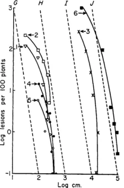
Equation 12 was used only to build up an argument. In scrapping it one need not replace it by a better equation, but only consider its most useful features. The central inferences from the equation concern the value b = 2, or, to scrap the equation, concern a gradient in which the number of lesions formed by inoculum from a source varies inversely as the square of the distance from the source. If one plots the number of lesions against distance on a log-log scale, the inverse-square lines are straight. One can draw as many as one wishes—all parallel. Such are the lines A, B, C, D in Fig. 3. The observed gradient for any disease can then be compared immediately with these lines. If its slope is steeper than theirs, there will be a horizon of infection, and spread will be continuous. Similarly one can draw a number of parallel inverse-cube lines like the lines Ε and F in Fig. 3. If the observed gradient is steeper than theirs, horizons can be expected to be fairly close. In Fig. 4 the process is continued, and lines G, Η, 7, and / show the number of lesions inversely as the fourth power of the distance from the source of infection.
Dutch elm disease, caused by Ceratostomella ulmi, was chosen to illustrate Fig. 3. There is a fair amount of information about it. Among other things, the spread of disease from a single infected tree in a limited period of time has been observed by several workers to virtually cease within some hundreds of yards from the tree, so one knows in advance that one should expect gradients steeper than the inverse-square lines. On one point there is a difficulty—a difficulty common to most of the literature of diseases that could be used for illustration: gradients should be determined only at low percentages of disease. This limits information to the lower part of the curve; the disadvantage of this is that information there is usually based on relatively few diseased plants and is consequently not powerful statistically. At higher levels of disease one can correct the curve partially (or fully, if the lesions are distributed randomly) by transforming percentages of diseases into calculated numbers of infections per 100 plants. Attention to this was drawn by Gregory (1948), who published a useful table of transformed values.
Some examples will explain the transformation. Suppose there were exactly 100 random infections per 100 plants. Not all plants would be infected; on an average, 36.8% would have no infections (they would remain healthy) and 63.2% would have 1 or more infections. The table calculates this in reverse; it transforms 63.2% disease to 100 infections
per 100 plants. In Fig. 3 the highest figure for disease is 88.9%, which is transformed to 220 infections per 100 trees. At low percentages the change is small and usually negligible: 5% disease transforms to 5.13 infections per 100 plants.
Figure 3 analyzes the combined data of Zentmyer et al. (1944) for three plots in Connecticut; and the data of Liming et al. (1951) for a
I cm. 10 cm. I m. 10m. 100 m. I km.
Log cm.
FIG. 3 . Amount of Dutch elm disease (Ceratostomella ulmi) at varying dis
tances from the source of inoculum. Curves 1 and 2 : data of Zentmyer et al. ( 1 9 4 4 ) and Liming et al. ( 1 9 5 1 ) , respectively, shown as transformed numbers of infections.
A, B, C, and D are inverse-square lines with scales of distances as 1 : 1 0 : 1 0 0 : 1 0 0 0 . Ε and F are inverse-cube lines with scales of distance in the ratio 1 : 1 0 .
plot in New Jersey. These data were collected within a year of the emergence in large numbers of the vector beetles from the source of infection which in each case was a single naturally infected tree. There was therefore little time for secondary multiplication to affect the gradients. At the lower levels of disease, which are the safest to observe, the gradients are steeper than the inverse-square lines and are more like the inverse-cube lines. This is what one would expect from general